1
Introduction to Cone Beam Computed Tomography
Conventional Computed Tomography (CT)
General Information
Computed tomography (CT) is credited to Godfrey Hounsfield, who in 1967 wrote first about the technology and then created a unit in 1972. He was awarded the Nobel Prize in Physiology/Medicine in 1979. Conventional CT units are both hard-tissue and soft-tissue imaging modalities. The first CT, first generation, had a scan time of 10+ minutes depending on how much of the body was being imaged. The processing time would take 2½ hours or longer. All first-generation CT units were only a single slice. This means that one fan of radiation exposed the patient and would have to circle around the patient several times to cover the area of concern. Current CT units are fifth generation, or helical/spiral. The scan times have gone down to 20–60 seconds with a processing time of 2–20 minutes. The number of slices available is up to 64, 128, and 256. The more slices available makes it possible to scan more of the patient in one circle, hence the lower scan times. Conventional CT units work with the patient lying down on a table while being scanned. The table moves in and out of the bore to cover the area of concern. Once all the data are received, they are compiled to create a dataset. This dataset can be manipulated to look at the information in many different angles.
Cone Beam Computed Tomography (CBCT)
General Information
Cone beam computed tomography (CBCT) was discovered in Italy in 1997. The first unit created was the NewTom. The NewTom was similar to conventional CT having the patient lying down with an open bore where the radiation exposes the patient. Instead of a fan of radiation (used in conventional CT units), a cone of radiation is used to expose the patient, hence the name cone beam computed tomography. As new CBCT units were created, companies started using seated or standing options. With continued updates to the units, the sizes have become smaller, with many needing only as much space as a pantomograph machine.
Conventional CT Versus Cone Beam CT
Voxels
Voxels are three-dimensional data blocks that representing a specific x-ray absorption. CBCT units capture isotropic voxels. An isotropic voxel is equal in all three dimensions (x, y, and z planes) producing higher resolution images compared to conventional CT units. Conventional CT unit voxels are nonisotropic with two sides equal but the third side (z-plane) different. The voxel sizes currently available in CBCT units range from 0.076 mm to 0.4 mm. The voxel sizes currently available in conventional CT units range from 1.25 mm to 5.0 mm. Resolution of the final image is determined by the unit’s voxel size. The smaller the voxel size the higher the resolution. However, the higher the resolution, the higher the radiation dose to the patient as well.
Field of View
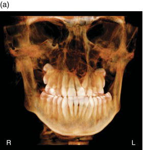
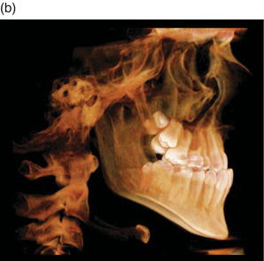
Field of view (FOV) is the area of the patient irradiated. CBCT units vary, with some units having a fixed FOV and some having changeable FOVs. The ranges of FOVs are from 5 cm × 3.8 cm, commonly referred to as a small FOV, to 23 cm × 26 cm, commonly referred to as a large FOV (Figures 1.1 to 1.3).
Radiation Doses
Radiation doses with CBCT units are as varied as the field of view options. CBCT units have approximate radiation dose ranges of 12 microSieverts to 1073 microSieverts. Conventional CT units have much higher radiation doses due to their soft tissue capabilities with doses of 1200 microSieverts and higher per each scan, depending on the selected scan field.
Figure 1.1. (a) 3D rendering of a small FOV of 5 cm × 8 cm from an anteroposterior (AP) view; (b) 3D rendering of a small FOV of 5 cm × 8 cm from a lateral view.
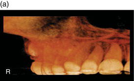
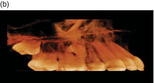
Figure 1.2. (a) 3D rendering of a medium FOV of 8 cm × 8 cm from an anteroposterior (AP) view; (b) 3D rendering of a medium FOV of 8 cm × 8 cm from a lateral view.
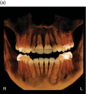
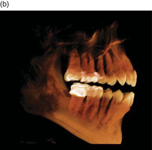
Figure 1.3. (a) 3D rendering of a large FOV of 16 cm × 16 cm from an anteroposterior (AP) view; (b) 3D rendering of a large FOV of 16 cm × 16 cm from a lateral view.
Viewing CBCT Data
Multiplanar Reformation (MPR)
Multiplanar reformation, or MPR, is a view frequently of three different directional 2D images (axial, coronal, and sagittal planes) (Figure 1.4). Within this view, the images may be manipulated in the thickness of data, and direction of viewing can be altered. Reconstructed pantomographs and lateral cephalometric skulls (Figures 1.5 and 1.6) are possible without distortion from standard 2D radiography. The dataset may also be manipulated to create cross-sectional (orthogonal) views of the jaws and condyles (Figures 1.7 and 1.8).
3D Rendering
The most common form of 3D rendering offered in CBCT software is indirect volume rendering, which determines the grays of the voxels to create a 3D image (Figure 1.9). Another form of 3D rendering is referred to as direct volume rendering, or maximum intensity projection (MIP) (Figure 1.10).
Figure 1.4. Axial (A), sagittal (S), and coronal (C) views.
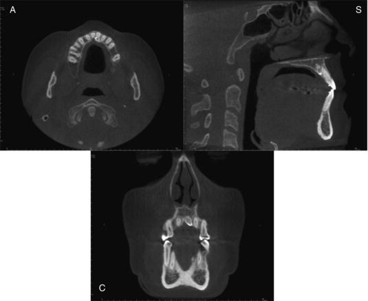
Figure 1.5. Sample reconstructed pantomograph with 3D view on bottom left, focal trough bottom middle, and preview on bottom right.
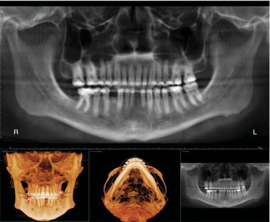
Figure 1.6. Sample reconstructed lateral cephalometric skull.
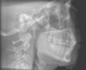
Figure 1.7. Sample cross-sectional slices with axial view and reconstructed pantomograph.
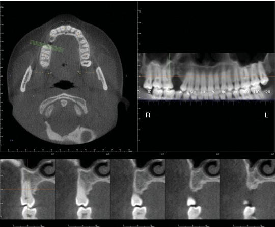
Figure 1.8. Sample temporomandibular joint view with cross-sectional slices.
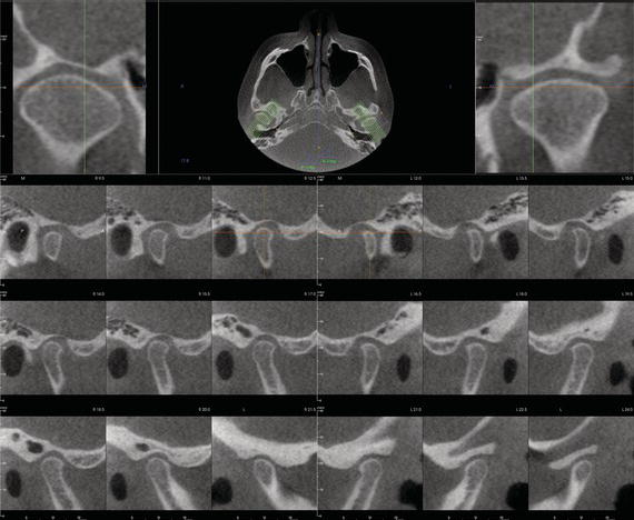
Figure 1.9. (a) 3D rendered view with teeth setting; (b) 3D rendered view with bone setting.
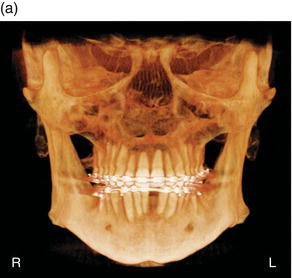
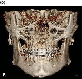
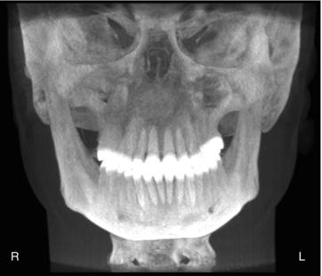
Figure 1.10. MIP view.
Stay updated, free dental videos. Join our Telegram channel
VIDEdental - Online dental courses


