Cone-beam computed tomography (CBCT) has become a popular modality in research, but it can be misused and misunderstood. Several image quality, bone biology, and statistical factors must be considered before designing CBCT studies or interpreting their results. Studies making small measurements, such as changes in buccal bone thickness, are especially susceptible to these factors. The spatial resolution as determined by a line pair phantom, the CBCT settings used, and a statistical power analysis should be reported in studies that investigate small bony changes. Protocols should therefore be established and followed to minimize the misinterpretation of results and improve the quality of research in this field.
Cone-beam computed tomography (CBCT) has become a popular modality in the evaluation of orthodontic diagnoses and outcomes. It offers high diagnostic value with a relatively low radiation dose. Its linear accuracy has also been verified. This accuracy has justified the use of CBCT scans in studying implant sites, palatal thickness, and cephalometrics. Thus far, these studies have been limited to larger measurements spanning severalcentimeters.
Recently, there has been interest within the research community in using CBCT to evaluate smaller maxillofacial structures: in particular, buccal-bone thickness before, during, and after treatment. Before one undertakes or interprets a study evaluating buccal bone with CBCT, several image quality, bone biology, and statistical factors must be considered.
Spatial resolution is the minimum distance needed to distinguish between 2 objects and is often incorrectly assumed to be equal to a scan’s reported resolution or voxel size. Factors such as partial volume averaging, noise, and artifacts make it impossible to achieve a resolution equal to the voxel size. These factors and others will be discussed in this article.
In a study by Ballrick et al, a Classic i-CAT (Imaging Sciences International, Hatfield, Pa), set at 120 kVp and 5 mA, was used with a line pair phantom to test the spatial resolution of all potential field of view (FOV) and voxel size combinations. Those authors found that a 0.2 mm voxel scan had an average spatial resolution of 0.4 mm. The 2 most common voxel sizes used for orthodontic scans—0.3 and 0.4 mm—both averaged a spatial resolution of 0.7 mm. In areas of thin bone, a spatial resolution of 0.7 mm would not be adequate to properly visualize the bone.
Spatial resolution is also frequently confused with measurement accuracy. Measurements made with CBCT have been shown to be accurate to within 0.1 to 0.2 mm. However, linear accuracy over long distances is different from a scan’s ability to differentiate between 2 objects in close proximity (spatial resolution).
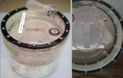
Because of the multi-factorial nature of spatial resolution, each machine and scan must be evaluated individually. For CBCT studies that focus on small measurements, it would be prudent to use a line pair phantom ( Fig 1 ) to determine the unique spatial resolution of the machine and the scan settings used. Caution should be exercised when drawing conclusions based on numbers smaller than a scan’s spatial resolution. If a study fails to report a scan’s spatial resolution and, instead, simply reports the voxel size, we are left without the proper tools to interpret the results. Also, spatial resolutions determined using the ideal conditions in a phantom will always overestimate the subsequent in-vivo spatial resolution.
An important factor influencing in-vivo spatial resolution is partial volume averaging. Frequently, the size of a voxel is larger than the object or the densities it represents. This occurs most often along the margin of an object or at the boundary of 2 substances of differing densities. The voxel can display only 1 gray value at a time. To account for this, the voxel displays an average of the densities present. Simply put, if a voxel represents an area of 75% lucent soft tissue and 25% opaque cortical bone, the voxel will appear more lucent than opaque. This process can make boundaries between densities harder to accurately distinguish, and results in lower spatial resolution.
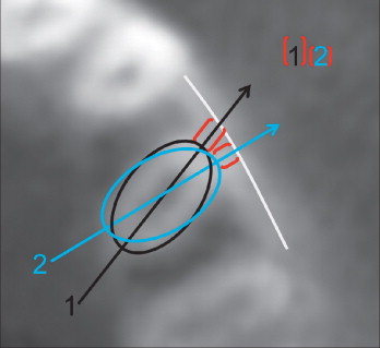
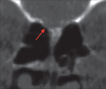
Thin bone is especially susceptible to partial volume averaging, not just buccal bone, but also with areas such as temporal bone and the sphenoid sinus ( Fig 2 ). The affect of partial volume averaging on thin bone has been well documented in conventional computed tomography (CT) scanners. It was shown that the angle at which the image plane intersects the bone wall can cause thin bone to appear thicker or thinner than it truly is. This type of partial volume averaging can cause bone walls thinner than 1 mm to all but disappear on CT scans.
The most effective way to decrease the influence of partial volume averaging is to decrease the voxel size. There is a trade-off, however, when using smaller voxel sizes, since they require more radiation and are more prone to noise.
Noise is the result of unintended energy or photons hitting the detector and clouding the resultant image. The noise levels in scans vary greatly between machines. Some machines have cleaner or less noisy images, whereas others are more difficult to read. Each machine’s settings, environment, and reconstruction algorithms affect the image’s noise.
A main cause of noise in a scan is scatter radiation. Compared with medical CT, CBCT can have up to 15 times higher scatter levels. Medical CT’s lower scatter levels allow it to image some structures better than CBCT. For example, Loubele et al found that medical CT is superior to CBCT in imaging cortical bone.
In CBCT, scatter levels increase as the size of the FOV increases. The easiest way to decrease noise from scatter is to use the smallest FOV that encompasses the region of interest. The larger the FOV and the greater the scatter, the worse the spatial resolution becomes. For this reason, large FOVs, such as those frequently used in orthodontic scans, are contraindicated for clinicians wishing to evaluate buccal bone thickness.
Smaller FOVs may decrease noise from scatter, but decreasing the voxel size has an inverse effect. As voxels decrease in size, they become more sensitive to noise, resulting in poorer spatial resolution than one might expect. Reconstruction algorithms can decrease the noise in small voxel scans but require further development. Although a voxel size of 0.125 mm is available, because of noise and other factors, a spatial resolution of 0.125 mm is currently unachievable.
A number of artifacts can affect the quality of a CBCT image. The most apparent ones in orthodontics are metal artifacts. CBCT scans taken with braces present show streaking artifacts around the teeth ( Fig 3 ). These artifacts might simply be a nuisance, except that they can affect how a scanner interprets and reconstructs the surrounding structures. Katsumata et al showed that the densities of surrounding structures can affect an adjacent voxel’s perceived density. For this reason, a practitioner should be cautious in making measurements close to braces or other metal objects, since the spatial resolution in that area will be compromised. An analogy would be trying to spot an airplane flying close to the sun. The closer the airplane gets to the sun, the harder it becomes to see because of the sun’s brightness. The airplane is still there, but the sun has made it difficult to distinguish.
Another artifact frequently encountered in orthodontics is movement. CBCT is more sensitive to patient movement than medical CT. The most effective way to limit movement artifacts is to decrease the scan time. This is especially helpful with younger orthodontic patients. However, with a decreased scan time comes fewer data or frame acquisitions. This leads to undersampling, which makes resolving fine details difficult.
This presents a dilemma when the goal of the scan is to achieve high spatial resolution. Do you expose the patient to a longer scan to improve spatial resolution but increase the risk of movement artifacts? Or do you compromise spatial resolution to decrease the risk of movement artifacts? Most orthodontic scans are taken with a short scan time, resulting in fewer frames acquired, fewer movement artifacts, and lower spatial resolution. Orthodontic scans with these characteristics are ideal for general treatment planning but should be used with caution if the goal is to properly evaluate the fine details of the buccal bone.
Image quality is also affected by the gray scale bit depth of the CBCT system used. Current CBCT systems range from 12-bit to 16-bit gray scale. Since the human eye cannot distinguish beyond 10-bit gray scale and computer monitors are currently available in only 8-bit or 10-bit gray scale, some people assume that it would not be worthwhile to exceed these thresholds. However, this approach fails to take into account that the reconstruction software uses the increased bit depth to improve its primary and secondary reconstructions, resulting in a cleaner and more defined volume. Most software also allows the clinician to change the values of gray scale displayed on the screen using a process called windowing. By scrolling through the various values of gray captured in the scan, the clinician can better visualize the volume. In essence, the software allows us to use the additional shades of gray captured by the scan despite the limitations of our eyes and computer monitors. When evaluating small structures, the highest available gray scale should be used.
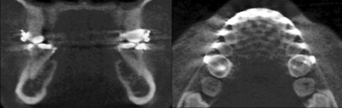
Moving beyond image quality, another consideration is the orientation and location of the image planes used to visualize the region of interest. Since most crowded teeth have some rotation, the thinnest portion of bone might not correspond to the buccal surface of the root. A rotated tooth will naturally have thicker bone along the buccal surface of its root. However, when the tooth is derotated, the buccal surface of the root will move into thinner bone ( Fig 4 ). This phenomenon can easily be mistaken for bone loss, whereas in reality the buccal surface of the root has simply rotated into a new bony position. For this reason, buccal bone measurements should be made at several sites around the tooth and averaged for a more honest representation of bone support regardless of the tooth’s rotation. If the measurement is made only at the buccal surface of the root at both pretreatment and posttreatment times, the derotated tooth will appear to be in thinner bone after treatment.