Introduction
The purpose of this study was to evaluate the accuracy and reliability of cone-beam computed tomography (CBCT) in the diagnosis of naturally occurring fenestrations and bony dehiscences. In addition, we evaluated the accuracy and reliability of CBCT for measuring alveolar bone margins.
Methods
Thirteen dry human skulls with 334 teeth were scanned with CBCT technology. Measurements were made on each tooth in the volume-rendering mode from the cusp or incisal tip to the cementoenamel junction and from the cusp or incisal tip to the bone margin along the long axis of the tooth. The accuracy of the CBCT measurements was determined by comparing the means, mean differences, absolute mean differences, and Pearson correlation coefficients with those of direct measurements. Accuracy for detection of defects was determined by using sensitivity and specificity. Positive and negative predictive values were also calculated.
Results
The CBCT measurements showed mean deviations of 0.1 ± 0.5 mm for measurements to the cementoenamel junction and 0.2 ± 1.0 mm to the bone margin. The absolute values of the mean differences were 0.4 ± 0.3 mm for the cementoenamel junction and 0.6 ± 0.8 mm for the bone margin. The sensitivity and specificity of CBCT for fenestrations were both about 0.80, whereas the specificity for dehiscences was higher (0.95) and the sensitivity lower (0.40). The negative predictive values were high (≥0.95), and the positive predictive values were low (dehiscence, 0.50; fenestration, 0.25). The reliability of all measurements was high (r ≥0.94).
Conclusions
By using a voxel size of 0.38 mm at 2 mA, CBCT alveolar bone height can be measured to an accuracy of about 0.6 mm, and root fenestrations can be identified with greater accuracy than dehiscences.
Despite many reports in the literature on the various uses of cone-beam computed tomography (CBCT), studies on its accuracy and image quality for assessing bone morphology have been limited. Also, no studies have assessed the use of CBCT to study alveolar bone morphology in vivo. Instead, most studies used radiographic phantoms, which do not accurately represent some anatomic structures such as tooth sockets and alveolar bone margins. Other studies have used human skulls, but the defects measured were created by the operator. Still other studies compared CBCT to multi-slice spiral computed tomography, multidetector-row helical computed tomography, or spiral computed tomography as gold standards. The problem with comparing CBCT to other computed tomography (CT) machines is that all have some measurement errors. In addition, multi-slice spiral CT, multidetector-row helical CT, and spiral CT use more radiation and have higher costs, limiting their use for routine dentalradiography.
The first model of CBCT that used a cone-beam x-ray instead of the traditional fan beam was the dynamic spatial reconstructor introduced by Hoffman et al and Ritman et al in 1980. This was developed to image a volume instead of a slice as in conventional CT with “stop-action” pulsed radiation to minimize blurring effects from motion and high-temporal resolution that were especially important for imaging the heart, lungs, and circulation. Although the high temporal resolution of the dynamic spatial reconstructor was useful in angiographic imaging with contrast agents, the volumetric anatomic structures generated were indistinct. Additionally, the unit was not readily accessible, since it was expensive and weighed 13 tons. Over the past few decades, the dynamic spatial reconstructor evolved into the current CBCT that uses less expensive x-ray tubes, along with more powerful personal computers and higher-quality detectors, allowing for relatively low radiation doses and smaller size requirements for operation, making CBCT more affordable and feasible in smaller clinical officesettings.
According to the definition of Carranza et al, fenestrations are isolated areas in which the root is denuded of bone, and the root surface is covered only by periosteum and overlying gingiva. Dehiscencesare bony defects in which the denuded areas involve the alveolar bone margin. The presence of these buccal alveolar bone defects decreases the bony support for the teeth. It is well documented that, under certain conditions (eg, plaque-induced inflammation), a lack of bony support during orthodontic movement can be detrimental to the health of the teeth and the periodontium. In addition, orthodontic tooth movement can create alveolar bone defects. Until recently, bony dehiscences and fenestrations could not be visualized by traditional 2-dimensional radiography because of the superimposition of contralateral cortical bony or dental structures. The development of CT and especially CBCT has provided the means to visualize these defects 3 dimensionally. The literature has reported the accuracy of CT and CBCT for measuring and identifying artificially created alveolar bone defects. However, no studies have evaluated the use of CBCT to diagnose naturally occurring bony dehiscences and fenestrations in human skulls. Also, no studies have determined the positive and negative predictive values when CBCT is used to diagnose alveolar bone defects. The purposeof this study was to evaluate the accuracy and reliability of CBCT in the diagnosis of naturally occurring fenestrations and bony dehiscences.
In addition, we evaluated the accuracy and reliability of CBCT to measure the alveolar bone margins on dentate skulls. This is important because the identification of these alveolar bone defects before orthodontic treatment is helpful for the clinician when planning treatment. An undiagnosed buccal alveolar bone defect could occur in a few patients and cause greater potential for treatment relapse or gingival recession resulting in an unesthetic finish of orthodontic treatment. The first hypothesis was that there is no difference in the measurement of alveolar bone height with CBCT compared with physical measurements. The second hypothesis was that there is no difference in the detection of dehiscences and fenestrations with a CBCT imaging system compared with direct assessments on dry human skulls.
Material and methods
Dry human skulls were selected from the Hamann-Todd skull collection at the Bolton-Brush Growth Study and the Museum of Natural History in Cleveland, Ohio. A preliminary screening of 39 skulls including 1040 teeth showed that the prevalences of dehiscences and fenestrations were approximately 11% and 8% of these teeth, respectively. These percentages were equivalent to the average of the rates reported in the literature. A sample size estimate for a descriptive study by using proportions was determined to be 240 at confidence intervals of 99% and 1%. In addition, the sample size calculation for comparison of 2 groups by using a standardized effective size of 0.25 mm based on previous studies at a 5% level of significance and an 80% power was found to be a minimum of 240. A sample of 13 skulls with 334 teeth was selected with these inclusion criteria: (1) adult skulls based on dentition,(2)intact skulls with both the maxilla and the mandible, (3)minimum of 10 teeth per jaw, (4) no obvious pathology (cyst or tumor in the alveolar process), and (5) no mechanical damage (chips, cracks, or breaks in the alveolarprocess).
The skulls were scanned by using a commercially available CBCT scanner (CB MercuRay, Hitachi Medical Systems American, Twinsburg, Ohio). After ensuring that the machine’s calibration was correct, the skulls were positioned in the center of the scanning table in the same orientation as a live patient by using vertical and horizontal light guides ( Fig 1 ). To allow visualization of both maxillary and mandibular cusps, the maxillary and mandibular dentitions were discluded with a cotton roll at the anterior region. The scanning parameters for imaging were 110 kVp, 2 mA, 9.6 seconds per revolution, and a12–in field of view (FOV) (F mode). These settings produced a voxel size of 0.38 mm. The settings were the same as those used for orthodontic diagnosis and treatment planning in the graduate orthodontic clinic at Case Western Reserve University.
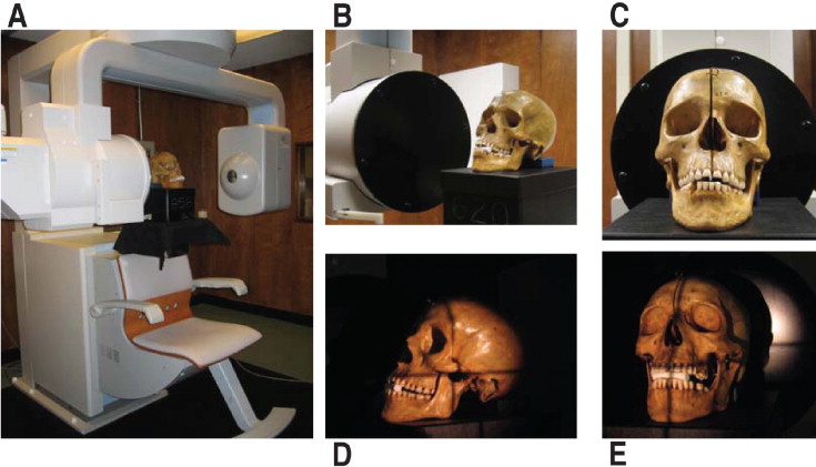
Raw data were collected and reconstructed into 3-dimensional (3D) volumes by using the software from the manufacturer. The reconstructed data were exported and saved as digital imaging and communications in medicine (DICOM) files. The 512 two-dimensional slices were imported into a commercially available software program (Accurex, version 1.1, Cybermed, Seoul, Korea) on a networked computer workstation (Windows NT, Dell, Round Rock, Tex) for 3D volume rendering. The 3D volume-rendering mode was used to display the CBCT images for evaluation and analysis. The radiodensity in Hounsfield units (HU) was adjusted by the operator to the threshold deemed optimal for visualization of the buccal alveolar bone ( Fig 2 ). Based on a preliminary skull study, the threshold window was fixed for all skulls at −280 and −510 HU at the upper and lower limits, respectively.
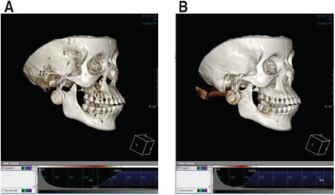
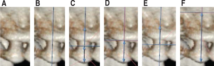
Figure 3 illustrates the measuring technique for the CBCT images. All measurements were made by the same operator (C.C.L.). Because of the tendency for fenestrations and dehiscences to occur on the labial and buccal surfaces, all measurements on the CBCT images were made on the buccal surface parallel to the long axis of the tooth. The first reference point was the cusp tip (T) for the posterior dentition and the midincisal tip (T) for the anterior dentition. The second reference point was the cementoenamel junction (CEJ) for the first measurement, the alveolar bone margin (BM) for the second measurement, and, if there was a fenestration, the coronal border of the fenestration for the third measurement (T-Fen1) and the apical border for the fourth measurement (T-Fen2). Since each molar has at least 2 buccal cusps, the mesiobuccal and the distobuccal cusps were measured individually. Table I describes the variables used. Previous studies used varying criteria for the identification of dehiscences, ranging from any defect greater than 1 mm near the CEJ, to 4 mm apical to the interproximal bone crest, to exposure of half of the root. In this study, to distinguish a dehiscence from horizontal bone loss caused by periodontal disease, a dehiscence was defined as a V-shaped defect along the BM, with the distance between the CEJ and the alveolar bone height 3 mm or greater. If a fenestration or dehiscence was found on the 3D volumetric view, it was further analyzed by using the 2-dimensional slice data to verify the presence or absence of bone covering the root surface. Defects were recorded if no bone could be seen covering the root surface when examining the axial and coronal slices at the heights indicated by T-BM for dehiscences, and between T-Fen1 and T-Fen2 for fenestrations.
| Variable | Description |
|---|---|
| Dehiscence | Buccal or facial alveolar bone defect involving an alveolar margin 3 mm or greater and concurrent with a V-shaped BM. |
| Periodontal recessions involving the interproximal bone were excluded. | |
| Fenestration (Fen) | A circumscribed defect on the buccal or facial alveolar bone exposing the root. |
| T-CEJ | The distance from the cusp tip to the CEJ parallel to the long axis of the tooth. Buccal cusps were used for posterior teeth and midincisal tips were used for anterior teeth. |
| T-BM | The distance from the cusp tip to the most coronal bone margin measured along a line parallel to the long axis of the tooth. |
| T-Fen1 | The distance from the cusp tip to the most coronal border of a fenestration along a line parallel to the long axis of the tooth. |
| T-Fen2 | The distance from the cusp tip to the most apical border of a fenestration along a line parallel to the long axis of the tooth. |
| Bone height | The distance obtained from taking the difference between the measurements T-CEJ and T-BM. the reference points were the same for a dehiscence. |
| Dehiscence height | The distance obtained from taking the difference between the measurements T-BM and T-CEJ. |
| Fenestration height | The distance obtained from taking the difference between the measurements T-Fen1 and T-Fen2. |
The same measurements were made directly on the skulls with a digital caliper calibrated to the nearest 0.01 mm (code no. 500-171-20, model no. CD-6-in CX Digimatic Caliper, Mitutoyo American, Plymouth, Mich). To limit experimental bias, all measurements on the skulls were done at least 2 weeks after the CBCT measurements. Table II shows the distribution of the teeth examined by tooth type. One hundred sixty-seven teeth were examined in both the maxillae and mandibles for a total of 334 teeth. A total of 446 measurements were made, since 2 reference points (mesial and distal cusps) were measured on the molars.
| Tooth type | Maxilla | Mandible | Total |
|---|---|---|---|
| Third molar | 17 | 7 | 24 |
| Second molar | 23 | 23 | 46 |
| First molar | 23 | 22 | 45 |
| Second premolar | 25 | 23 | 48 |
| First premolar | 22 | 25 | 47 |
| Canine | 21 | 21 | 42 |
| Lateral incisor | 22 | 23 | 45 |
| Central incisor | 14 | 23 | 37 |
| Total | 167 | 167 | 334 |
Statistical analysis
All statistical analyses were performed with the Statistical Package for Social Sciences (version 16.0, SPSS, Chicago, Ill). All linear measurements were adjusted for a known systematic software measurement error that underestimated the distance between 2 points by half of a voxel at each endpoint. Therefore, 0.38 mm was added to each measurement to correct for this software error. For a complete discussion of this systematic error, see the study of Baumgaertel etal. Measurement accuracy was evaluated by comparing the means, mean differences, and absolute mean differences for linear measurements. Two-tailed paired t tests were used to examine differences between means, and Pearson correlation coefficients were used to estimate the relationship between the direct (digital caliper) and indirect (CBCT) methods. A P value of ≤0.05 was used to assign statistical significance. Categorical data (presence or absence of fenestrations and dehiscences) were analyzed by using 2 × 2 tables, and the sensitivity, specificity, and positive and negative predictive values were calculated for both direct and indirect (CBCT) methods. The direct method was used as the gold standard for comparison.
To determine the reliability of the methods, 65 randomly selected teeth (91 sites) were reexamined and remeasured with both methods at least 2 weeks after the initial measurements. The intraoperator reliability was assessed by calculating the intraclass correlation coefficient (ICC) between measurements collected at bothtimes.
Results
The linear measurement accuracy of CBCT was demonstrated by the means, mean differences, and absolute mean differences between each pair of direct and CBCT measurements. Pearson correlation coefficients were also calculated for each pair of direct and indirect measurements. Table III shows these descriptive statistics for measurements of T to CEJ and T to BM for all sites examined. The means for both CBCT and direct T-CEJ measurements were approximately equal (8.3 ± 1.4 vs 8.3 ± 1.5 mm), and the mean differences between the 2 methods showed that the CBCT measurements were essentially equal to the direct measurements (−0.1 ± 0.5 mm). The absolute mean differences showed a difference of 0.4 ± 0.3 mm between the CBCT and direct measurements; this was about the size of a voxel. The linear measurement, T-BM, was 0.2 ± 1.0 mm smaller on average for CBCT, and the absolute mean difference was 0.6 ± 0.8 mm. Paired t tests showed a significant difference between CBCT and direct measurements to both CEJ and BM ( P ≤0.01). The correlation between CBCT and direct methods for T-CEJ measurements was high (r = 0.94) as was the correlation for T-BM at 0.87.
| Variable | Direct Mean ± SD (mm) | CBCT Mean ± SD (mm) | Difference (direct-CBCT) Mean Diff ± SD * | Difference (direct-CBCT) Mean Abs ± SD † | Correlation | Significance |
|---|---|---|---|---|---|---|
| T-CEJ | 8.3 ± 1.5 | 8.3 ± 1.4 | −0.1 ± 0.5 | 0.4 ± 0.3 | 0.941 ‡ | 0.002 § |
| T-BM | 10.3 ± 2.1 | 10.6 ± 1.9 | −0.2 ± 1.0 | 0.6 ± 0.8 | 0.871 ‡ | 0.000 § |
* Mean difference between each direct and CBCT measurement.
† Mean of the absolute difference between each direct and CBCT measurement.
‡ Pearson correlation coefficient is significant at the 0.01 level.
The number of fenestrations detected by CBCT was more than 3 times higher than for direct examination (104 fenestrations by CBCT vs 32 by direct measurement; Table IV ). The number of dehiscences was less for CBCT than for direct (43 dehiscences vs 52). Fenestrations were detected more often in the maxilla than in the mandible for both CBCT and direct measurements, whereas dehiscences were detected more often in the mandible than in the maxilla.
| Direct | CBCT | ||||
|---|---|---|---|---|---|
| Tooth type | Sites (n) | Fenestrations | Dehiscences | Fenestrations | Dehiscences |
| Maxilla | 230 | 24 | 22 | 81 | 16 |
| Third molar | 34 | 2 | 1 | 3 | 1 |
| Second molar | 46 | 0 | 0 | 3 | 0 |
| First molar | 46 | 12 | 6 | 32 | 5 |
| Second premolar | 25 | 0 | 3 | 10 | 1 |
| First premolar | 22 | 2 | 4 | 13 | 4 |
| Canine | 21 | 4 | 7 | 5 | 4 |
| Lateral incisor | 22 | 3 | 0 | 9 | 1 |
| Central incisor | 14 | 1 | 1 | 6 | 0 |
| Mandible | 216 | 8 | 30 | 23 | 27 |
| Third molar | 13 | 0 | 0 | 0 | 0 |
| Second molar | 44 | 0 | 1 | 0 | 2 |
| First molar | 44 | 0 | 2 | 1 | 3 |
| Second premolar | 23 | 1 | 1 | 4 | 2 |
| First premolar | 25 | 2 | 7 | 2 | 7 |
| Canine | 21 | 1 | 5 | 7 | 5 |
| Lateral incisor | 23 | 2 | 8 | 5 | 6 |
| Central incisor | 23 | 2 | 6 | 4 | 2 |
| Total | 446 | 32 | 52 | 104 | 43 |
The CBCT and direct results were analyzed by using 2 × 2 contingency tables ( Table V ). For fenestrations, the sensitivity and specificity of CBCT were both at 0.81 ( Table VI ). For dehiscences, the specificity of CBCT was 0.95, and the sensitivity was 0.42. The negative predictive value for fenestrations, the probability that a negative test result (absence of fenestration) was truly negative, was 0.98, whereas the positive predictive value, the probability that a positive test result (presence of fenestration) was truly positive, was only 0.25. The negative predictive value for dehiscences was 0.93, and the positive predictive value was only 0.51. Sixteen false-positive dehiscences were excluded by examining axial and coronal slices, and 2 true-positive dehiscences were eliminated. For fenestrations, 57 false positives were excluded when slice data were examined, and no true positives were eliminated ( Table VI ).
| Fenestrations | Dehiscences | ||||
|---|---|---|---|---|---|
| Direct | Direct | ||||
| Fen + | Fen – | CBCT | Deh + | Deh – | |
| CBCT | |||||
| Fen + | 26 | 78 | Deh + | 22 | 21 |
| Fen – | 6 | 336 | Deh – | 30 | 373 |
Stay updated, free dental videos. Join our Telegram channel
VIDEdental - Online dental courses


