Material and methods

Six skeletally mature female foxhound mixes, approximately 2 years of age and weighing between 55 and 65 pounds, were used for this study. Foxhound dogs are an established model for investigating peri-implant osseous dynamics; their large jaws allow for the placement of multiple MSIs. The Institutional Animal Care and Use Committee at Texas A&M University Baylor College of Dentistry in Dallas, Tex, approved the care of the animals and the experimental protocols.

The MSIs used (Neodent, Curitiba, Paraná, Brazil) were self-drilling and made of titanium alloy; the threaded portions were 5 mm long and 1.6 mm wide (outer diameter). The MSIs were fabricated to have threaded SmartPeg (Osstell AB) accepting heads. To prevent tissue overgrowth, each animal had 6 to 8 MSIs placed on the lingual surface of the mandible. MSIs were placed in the furcations and between the teeth, depending on space availability in each dog. Using random assignment, pairs of MSIs were placed in the same location in both sides of the mandible: one with a pilot hole and one without. The Osstell device (Osstell AB) was used to measure implant stability immediately after MSI placement and every week thereafter until the dogs were euthanized. Bony adaptation was evaluated 3 dimensionally with microcomputed tomography and histologically with fluorescence.

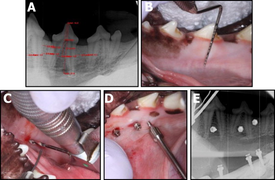
After quarantine and before MSI placement, all animals were sedated with ketamine (2.2 mg/kg intramuscularly) and rompin (0.22 mg/kg intramuscularly) and given a prophylaxis with ultrasonic scaling with chlorhexidine. On the day of MSI placement, periapical radiographs were taken bilaterally and measured to determine screw locations ( Fig 1 , A ). The animals were intubated and maintained with 1% isoflurane with oxygen at 1 L per minute. Radiographic measurements were transferred intraorally via a perio probe ( Fig 1 , B ), and the sites intended for MSI placement—interdental or interradicular—were marked. Local anesthetic (2% lidocaine with 1:100,000 epinephrine) was administered via local infiltration. A 1.1-mm drill bit (Neodent; 3M, St Paul, Minn) was used for the pilot holes. They were drilled at 1600 revolutions per minute all the way through the cortical bone under copious irrigation ( Fig 1 , C ). All MSIs were placed by hand ( Fig 1 , D ), with care taken to ensure that each pair of MSIs was screwed into the bone at the same level. Radiographs were taken again after placement to ensure proper MSI placement ( Fig 1 , E ). Both analgesics (torbugesic 0.2 mg/kg, 2 mg/mL with 1 mL per animal) and antibiotics (penicillin G 60,000 units/kg) were administered. For histologic evaluations of newly calcified bone, calcein was administered intravenously 2 weeks after MSI placement, and tetracycline was administered 5 weeks after placement.

A, Radiograph to determine sites for MSI placement in the mandible; B, measurements transferred to the site with a perio probe; C, pilot hole placement; D, MSI placement; E, postoperative radiograph confirming intraradicular and interdental placement of MSIs.

A total of 40 MSIs were placed (all as contralateral pairs of experimental and control), and the experiment lasted for 7 weeks. Thirty-four MSIs were placed at baseline; 2 MSIs (1 experimental, 1 control) were placed at 4 weeks to evaluate healing at its theoretical low point ; 4 more MSIs (2 experimental, 2 control) were placed when the dogs were killed (7 weeks). Inspection of MSIs and tissue conditions, administration of chlorhexidine gel, and Osstell ISQ measurements were performed weekly.

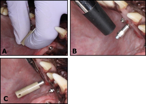
The Osstell Mentor uses an electromagnetic signal to measure the implant’s stability based on how much the SmartPeg vibrates. The Osstell device has been shown to be reliable for measuring MSI stability in vitro and in vivo. The SmartPeg was screwed into each MSI according to the manufacturer’s recommendations ( Fig 2 , A ). Four measurements—2 roughly parallel to the occlusal plane and 2 roughly perpendicular to the occlusal plane—were taken perpendicular to the long axis of the MSI and averaged ( Fig 2 , B ). The MSI was stabilized with a hemostat for SmartPeg insertion and removal ( Fig 2 , C ).

A, SmartPeg placement with SmartPeg Mount; B, measurement with Osstell ISQ; C, hemostat for SmartPeg removal.

At the completion of the 7-week experimental period, the dogs were euthanized, and the mandibles were disarticulated. Each bone-implant sample was retrieved with a modified 10-mm-diameter trephine bur (ACE Dental Implant System, Brockton, Mass) under copious irrigation. The samples were trephined parallel to the long axis of the implant to reduce scatter during scanning. Care was taken to ensure that all layers of the bone remained undamaged during the retrieval process. The samples were labeled and stored in 70% ethanol under limited lighting conditions.

When needed to ensure their precise fit into the cylindrical (9.8-mm internal diameter) sample holders used for scanning, a wet grindstone was used to smooth the outer edges of the bone-implant specimens. Four to 6 bone-implant specimens were placed in each holder, separated by sponges, and kept hydrated with 70% ethanol. The samples were evaluated using microcomputed tomography (modol 35; Scanco Medical, Bassersdorf, Switzerland) with an isotropic resolution of 6 μm. X-ray energy levels were set to 70 kVp, current to 114 μA, and integration time to 800 ms. A 0.5-mm aluminum filter and a high resolution setting of 1000 projections per 180° were used to ensure the highest quality scans with minimal metal implant artifact. The average scanning time was approximately 3.2 hours per specimen.

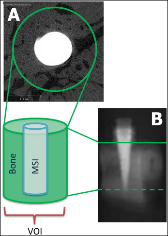
Cortical and trabecular volumes of interest were determined for each specimen. The volumes of interest were horizontally defined by circles drawn around the center of each MSI and perpendicular to the long axis of the MSI ( Fig 3 ). The coronal limit of the cortical volume of interest was visually defined as the first slice showing bone completely surrounding and contacting the MSI. The apical limit of the cortical volume of interest was visually defined as the most apical slice showing no trabecular bone (based on the absence of marrow spaces). The coronal limit of the trabecular volume of interest was defined visually as the most coronal slice with only trabecular bone surrounding the MSI; the apical limit was visually defined at the MSI apex ( Figs 3 and 4 ).

A, Original gray-scale 2-dimensional image with MSI in center ( white ), surrounding bone ( gray ), and space ( black ); the volume of interest ( VOI ) was defined with the MSI in the center. B, Coronal limit of the volume of interest visually defined as the first slice at which bone was observed completely surrounding and contacting the MSI.

Schematic description of the 3 (3-dimensional) BV/TV measurements evaluated: 6- to 24-μm ( white ), 24- to 42-μm ( purple ), and 42- to 60-μm segments ( red ). The 0 to 6 μm ( black ) segment was excluded from evaluation. Cortical and trabecular sections were evaluated for each bone-implant specimen.

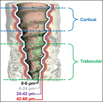
After scanning, a threshold (1 gray scale number, above which all voxels were considered to be bone, and below which all voxels were considered not to be bone) was determined based on multiple comparisons to distinguish the MSI from mineralized bone and background. Scanco Medical proprietary programming scripts with different parameters for BICs were processed for each sample. Separate bone volume to total volume fractions (BV/TV) were calculated for the cortical and trabecular volumes of interest. Based on previously established protocols, BV/TV values of 3 layers of bone surrounding the MSI were calculated. Each layer was 3 voxels (3-dimensional space with an associated gray-scale “brightness” value) thick, extending 6 to 24, 24 to 42, and 42 to 60 μm from the MSI surface ( Fig 4 ). BV/TV values of 0 to 6 μm from the MSI were excluded because of the metallic halation artifact.

Five pairs of bone-MSI specimens were evaluated histologically: 3 placed initially, 1 placed at 4 weeks, and 1 placed at 7 weeks that served as a control. They were dehydrated in graded alcohol over a period of 1 month and soaked in acetone for 3 days, methyl methacrylate monomer number 1 for 7 days, and methyl methacrylate monomer number 2 for 7 days. The samples were then embedded in methyl methacrylate until polymerization was complete. Serial sections of the samples were made. The slice that showed the greatest surface area of the MSI was polished and evaluated. The fluorescent signal was imaged using a fluorescent microscope (Nikon, Melville, NY) and a Photometrics CoolSnap K4 CCD camera (Roper Scientific, Duluth, Ga), and the signal was captured with NIS-Elements software (Nikon). Images were captured for calcein (green) using a filter with an excitation between 395 and 580 nm and an emission between 480 and 520 nm; the images for tetracycline (red) were captured using an excitation filter between 395 and 580 nm and an emission filter between 520 and 570 nm.

Results

All MSIs remained in place until the dogs were euthanized; none exhibited mobility. Four (10%) of the MSIs turned slightly (less than half a rotation) during placement or removal of the SmartPeg; none became unstable. The tissues around 11 of the 40 MSIs were inflamed at some point during the 7-week experimental period. This inflammation was usually due to food debris in or around the MSI head and usually resolved quickly, since the MSIs were irrigated and chlorhexidine gel was applied each week.

At placement and 1 week later, the MSIs with pilot holes showed significantly higher ISQ values than did the MSIs placed without pilot holes ( Table I ). The other ISQ values were generally higher for MSIs without pilot holes than for those with pilot holes, but no difference was statistically significant.

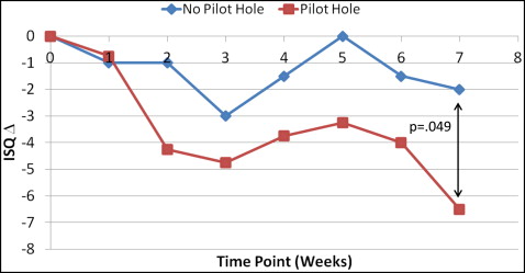
The median changes in ISQ values from baseline showed decreases during the first 3 weeks, increases over the next 2 weeks, and decreases over the last 2 weeks ( Fig 5 ). Although the decreases from baseline were generally greater for the MSIs with pilot holes than for those without pilot holes, only the difference at week 7 was statistically significant.

Median differences in ISQ from baseline.

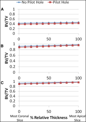
BV/TV increased slightly between the most coronal and apical slices of the cortical sections ( Fig 6 ). There was approximately 4% less cortical bone around MSIs with pilot holes than around those without pilot holes. At the most coronal aspect of the cortical sections, the only statistically significant difference occurred in the 6- to 24-μm layer, which showed 4.3% less bone around MSIs with pilot holes than without pilot holes ( Table II ). MSIs with pilot holes showed greater increases in BV/TV between the most coronal and apical slices than did those without pilot holes, resulting in even smaller differences in BV/TV at the more apical aspects of the cortical sections. Whereas all 3 cortical layers showed greater increases in BV/TV for the MSIs with pilot holes, only the differences in the 24- to 42-μm and the 42- to 60-μm layers were statistically significant.

Ratio of cortical bone volume to total volume (BV/TV) for A, the 6- to 24-μm layer; B, the 24- to 42-μm layer; and C, the 42- to 60-μm layer.

Table II

Multilevel estimates and standard errors of BV/TV fraction (%) for the 3 layers of cortical and trabecular bone around MSIs placed without pilot holes, with differences between those with and without pilot holes

	Layer (μm)	No pilot hole				Difference (no pilot hole – pilot hole)
		Constant		Linear		Constant		Linear
		Estimate	SE	Estimate	SE	Estimate	SE	Estimate	SE
Cortical	6-24	0.4258 ∗	0.0152	0.0405 ∗	0.0047	−0.0432 ∗	0.0216	0.0059	0.0075
	24-42	0.9197 ∗	0.0147	0.0546 ∗	0.0055	−0.0386	0.0210	0.0217 ∗	0.0087
	42-60	0.9355 ∗	0.0145	0.0441 ∗	0.0048	−0.0353	0.0207	0.0241 ∗	0.0077
Trabecular	6-24	0.3926 ∗	0.0234	−0.0815 ∗	0.0052	−0.1024 ∗	0.0330	0.1395 ∗	0.0068
	24-42	0.9195 ∗	0.0324	−0.2411 ∗	0.0068	−0.1361 ∗	0.0434	0.2215 ∗	0.0090
	42-60	0.9197 ∗	0.0334	−0.2312 ∗	0.0066	−0.1237 ∗	0.0428	0.2101 ∗	0.0088

Only gold members can continue reading. Log In or Register to continue

Share this:

• Click to share on Twitter (Opens in new window)
• Click to share on Facebook (Opens in new window)

Related

Related posts:

1. Ethics in orthodontics
2. It is all about definitions
3. Facial soft-tissue thickness in patients affected by bilateral cleft lip and palate: A retrospective cone-beam computed tomography study
4. Considering consideration
5. Clinical use of a direct chairside oral scanner: An assessment of accuracy, time, and patient acceptance
6. Can cone-beam computed tomography superimposition help orthodontists better understand relapse in surgical patients?

Stay updated, free dental videos. Join our Telegram channel

Join