20
Statistics As an Inductive Argument and Other Statistical Concepts
A judicious man looks at statistics not to get knowledge, but to save himself from having ignorance foisted upon him.
—Thomas Carlyle1
Statistics ≠ Scientific Method
Scientific method does not necessarily require the use of statistics. Indeed, papers published in areas such as molecular biology and biochemistry rarely use sophisticated statistics; the power of their experiment systems is so great that differences between the items being compared are evident enough not to require statistical tests. These differences may be observed directly (eg, the appearance or disappearance of a particular molecule that can be identified by its location on a polyacrylamide gel). This disclaimer notwithstanding, it should be noted that most clinical dental research does benefit from a statistical approach, because the size of the effects being observed is often small, and it is difficult to distinguish the effects from natural variation. The number of articles in the dental literature that employ statistics has risen rapidly, and instruction in statistics is now common—though not necessarily effective1—in dental schools.
The statistics used in most research papers are different from the statistics of everyday usage, such as reported census data or baseball batting averages that provide comprehensive information about the population involved. For example, in calculating a batting average, we know every time a player went to bat, and we know the player’s exact number of hits, so the batting average completely and accurately represents the player’s performance.
Statistical Inference Considered As an Inductive Argument
Golden rule of sample statistics
A number of features of statistical reasoning about samples were not illustrated in the previous chapters. Some of these may be summed up in what I will call the golden rule: Any sample should be evaluated with respect to size, diversity, and randomness.2 The statistics in research reports are based on samples. The obvious questions to ask are: (1) How representative of the target population are the samples? Was the sample selected randomly, or were there factors present that could lead to biased selection? (2) How large is the sample? (3) How much diversity exists in the sample? Does it cover all of the groups that make up the population? Fallacies, as well as acceptable arguments, can arise from statistical inference.
Fallacy of insufficient statistics (or hasty generalization)
In the fallacy of insufficient statistics, an inductive generalization is made based on a small sample.
| premise | My mother and my wife smoke. |
| conclusion | All women smoke (fallacy of insufficient statistics). |
If this argument were used as sole evidence for the conclusion that all women smoke, the argument would be classified as proof by selected instances.
Associated with this fallacy is the problem of how many is enough. The answer depends on how large, how varied, and how much at risk is the population being studied. Numbers that appear quite large can still be inadequate. Huff3 recounts a test of a polio vaccine in which 450 children in the community were vaccinated, while 680 were left unvaccinated as controls. Although the community was the locale of a polio epidemic, neither the vaccinated children nor the controls contracted the disease. Paralytic polio had such a low incidence—even in the late 1940s—that only two cases would have been expected from the sample size used. Thus, the test was doomed from the start.
What is a reasonable sample size?
There is no simple answer to this question, but two general considerations appear to be relevant: tradition and statistics.
Tradition
In some research areas, experience shows that consistent and reliable results require a certain number of subjects or patients; for example, Beecher4 recommends at least 25 patients for studies on pain. These traditions probably develop because of practical considerations such as patient availability, as well as inherent statistical considerations such as subject variability. The underlying philosophy in this approach is that the replication of results is a more convincing sign of reliability than a low P value obtained in a single experiment. If a number of investigators find the same result, we can have reasonable confidence in the findings. Means of combining and reviewing studies are given in Summing Up by Light and Pillemer.5
There are problems with the traditional method of choosing an arbitrary and convenient number of subjects. If the sample is too large, the investigator wastes effort and the subjects are unnecessarily exposed to treatments that may not be optimal. However, most often the number of subjects is too small; the size of the sample is usually limited by subject availability. Thus, studies that use low numbers of subjects and report no treatment effect should be considered with skepticism. In fact, some journals have a policy of rejecting papers that accept null hypotheses. Such negative results papers end up in a file drawer. They neither contribute to scientific knowledge nor enhance the careers of their authors. These “file-drawer papers” emphasize the need to understand the relationship between sample size and the establishment of statistically significant differences. Failure to use an appropriate sample size leads to much wasted effort.
Role of the sample size and variance in establishing statistically significant differences between means in the t test
The size of an adequate sample is a complex question that will not be addressed in great detail here. However, some insight into the problem can be gained by examining the formula for the t test, which is perhaps the most common statistical test used in biologic research. It should be used when comparing the means of only two groups. The t test exists in several forms that depend on whether the samples are related (eg, the paired t test) or independent. Below is the formula used for a two-sided comparison when comparing the means of the measured values from two independent samples with roughly equal variances of unpaired subjects:
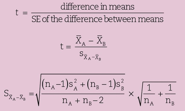
where nA, nB = number in samples A and B, respectively;  = means of samples A and B, respectively;
  = variance of groups A and B, respectively;
  = standard error (SE) of the difference between means; and nA + nB–2 = degrees of freedom.
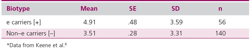
A high observed t value indicates the unlikeliness that the two samples are drawn from a population with the same mean. Having selected a significance level and calculated a quantity called degrees of freedom (df) (in this case df = nA + nB–2), we can consult a table of published t values such as can be found in appendix 3. If the observed t value is higher than the critical level, we reject the null hypothesis. For example, consider once again the study by Keene et al,6 who reported the decayed, missing, or filled teeth (DMFT) data found in Table 20-1:
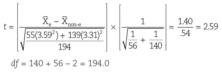
Table 20-1 Relationship of Streptococcus mutans biotype to DMFT*
The critical value of t for 194 df at an α level of .05 ≈ 1.96.
Since the calculated value of t = 2.59 > 1.96, we can reject the null hypothesis and conclude that there is a significant difference in DMFT between the e and non–e carriers.
From the formula for the statistic, we realize the following:
- A large difference between means will increase the t value. This makes sense. Large effects should be easier to see. If the effect is large, the sample size required to distinguish the groups will be smaller.
- The t value is decreased when the variance is large. (Remember that variance is related to the spread of measured values around the mean.) A large variance tends to produce a small t value, making it harder to detect differences between groups.
- The t value is increased when the number in the sample is large. From the formula, it can be calculated that the decrease in the SE value is proportional to the square root of the sample number. Thus, if you increase the sample size by a factor of 10, you only decrease the SE by 3.16. This may be an inefficient way of reducing the error, but it works. Bakan7 notes that increasing the sample size (n) almost inevitably guarantees a significant result. Even very small alterations in experiment conditions might produce minute differences that will be detected by a statistical test made very sensitive by a large sample size.
In the dental sciences, the reverse is the more common problem; that is, frequently there is only a small number in the sample. Combined with a large variability in the subjects, this small sample often means that no difference is detected, even when it is likely that a real difference exists.
Effect-size approach
Choosing the optimal sample size is a complex business that depends on the difference between groups, the variability of the groups, the experiment design, and the confidence level. A rough-and-ready way to estimate an appropriate sample size using the effect-size approach8 for a simple experiment with a treated and a control group follows:
- Estimate what you think is an important (or important to detect) difference in means between the treated and control groups.
- Use the results of a pilot study or previously published information on the measurement to estimate the expected pooled standard deviation (SD) of a reasonably sized sample.
- Using the values found in (1) and (2) above, calculate the d statistic (formula given on page 252).
- Choose your level of confidence (5% or 1%).
- Look up the number of subjects needed in appendix 6.
Using the same approach, we can also work backward to decide if a paper’s authors used a reasonable sample size. This is particularly important if no effect was seen, because the sample may have been too small to produce a sensitive experiment. To check this possibility:
- Use the authors’ data to estimate the d statistic.
- Look up the table in appendix 6 to determine the number of subjects that should have been used.
- Compare the number from the table with the actual number used. Effect- and sample-size tables for more sophisticated designs can be found in Cohen’s8 book Statistical Power Analysis for the Behavioral Sciences.
Dao et al9 examined the choice of measures in myofacial pain studies. Based on the characteristics of the measurements, they calculated how many subjects would be required to observe significant groups differing from each other by specified amounts. Their technique was based on the statistical power analysis developed by Cohen8 and is similar to the effect-size calculation given above. Their values for within- and between-subject variance were obtained from a population referred to as University Research Clinic. The technique used to measure pain was a visual analogue scale (VAS), shown to be a rapid, easy, and valid method that provides a more sensitive and accurate representation of pain intensity than the descriptive scales.
They found that detecting a 15% difference in pain intensity between treatment and control groups in an experiment with 3 groups would require 242 subjects per group. However, to detect an 80% difference in pain intensity, only 8 subjects per group would be needed, and the total study size would be 24 subjects. Even with the sensitive VAS method to measure pain, the traditional approach of using 25 subjects and descriptive scales could probably distinguish only very large differences between groups (ie, ≈ 80% differences, if three groups were used).
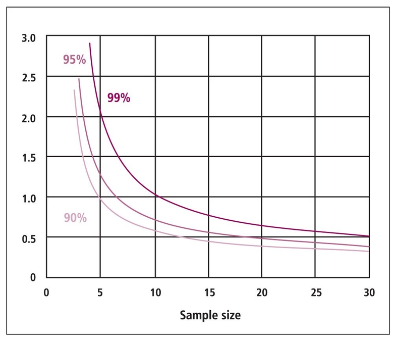
A handy rule for the effect of sample size on confidence intervals
Van Belle’s Statistical Rules of Thumb10 includes a chapter on calculating sample sizes and provides a number of other “rules of thumb” useful in performing practical statistical analysis. Figure 20-1, taken from van Belle,10 shows the half-width of confidence intervals with sample size. One can see that the width of the confidence interval decreases rapidly until 12 observations are reached and then decreases more slowly.
The Fallacy of Biased Statistics
To review briefly, descriptive statistics are simply efficient ways of describing populations. For our purposes, a population is a collection of all objects or events of a certain kind that—at least theoretically—could be observed. The specific group of objects (events, subjects) observed is the sample. Inferential statistics are concerned with the use of samples to make estimates and inferences about the larger population. This larger population from which the sample is selected is also called the parent population, or, perhaps more accurately, the target population. This is the population that we hope the sample represents, so that we can generalize our findings.
The fallacy of biased statistics occurs when an inductive generalization is based on a sample that is known to be—or is strongly suspected to be—nonrepresentative of the parent population. This problem of nonrepresentative samples is associated with the randomness of sample selection and the spread of the sample. Gathering numbers to obtain information may be likened to an archer shooting at a target. The bull’s-eye represents the true value of the population in question. The place where the arrow hits represents one value from the sample. Bias is the consistent repeated divergence of the shots from the bull’s-eye. For an archer, this bias may be caused by a factor such as a wind blowing from one direction that causes the arrows to hit predominantly on one side of the target. In research experiments, bias may be caused by factors leading to nonrandom sampling. There are many examples of biased polls giving erroneous results. Perhaps the most famous is the Literary Digest poll that predicted, on the basis of a telephone survey and a survey of its subscribers, that a Republican victory was assured in the 1936 election.3 The number of people polled was huge—over two million—but the prediction was wrong because the people polled were not representative of the voting public. In fact, they were wealthier than average because, at that time, telephones were found mainly in the homes of the wealthy. Thus, the Literary Digest poll selected relatively wealthy people, who stated that they would vote Republican. Today, the public opinion polls conducted by the Gallup and Harris organizations interview only about 1,800 persons weekly to estimate the opinions of US residents age 18 and over, but these polls are reasonably accurate because the sample is chosen by a stratified random sampling method that is not biased.
Bias can appear in many different ways, as denoted by Murphy’s11 definition:
Stay updated, free dental videos. Join our Telegram channel
VIDEdental - Online dental courses


