17
Correlation
The scientific literature is a large graveyard for correlations that didn’t “pan out” when more data became available.
—Peter A. Larkin1
The investigative strategies outlined in this chapter include: (1) cross-sectional survey; (2) ecologic study; (3) case-control design; and (4) follow-up (cohort) design.
Cross-sectional Survey
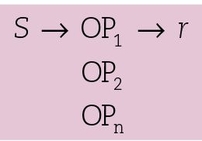
where S = pool of eligible subjects, OP1 = observation of property 1, OP2 = observation of property 2, OPn = observation of property n, and r = calculation of correlation coefficient or other measure of association.
As an example of a correlational cross-sectional study in dental research, consider the data from Keene et al1 in Table 17-1. The correlational strategy is used to relate two or more variables. Investigators classify the study subjects into groups and examine each subject individually to measure the different variables. In this example, investigators measured three properties: the Streptococcus mutans biotype; decayed, missing, or filled teeth (DMFT); and caries-free status. Often in cross-sectional studies, one variable is concerned with exposure (S mutans), while the other variables relate to “caseness” (ie, presence of some conditions). Each group member is then assigned a value, depending on the particular variable measured. The degree of relationship between the variables is then assessed with statistical techniques. Notice that because the Keene et al2 study is a correlational study, no attempt is made to manipulate the biotype of S mutans in the naval men. The biotype is simply measured. Hence, a correlational study is similar to the observation-description strategy and shares the same strengths and weaknesses. Two advantages of a simple correlational study (such as that of Keene et al2) are that (1) they are relatively inexpensive because no follow-up is required and (2) subjects are not exposed to potentially harmful agents or conditions.
Table 17-1 Correlation cross-sectional study measuring Streptococcus mutans biotype, DMFT, and caries prevalence*
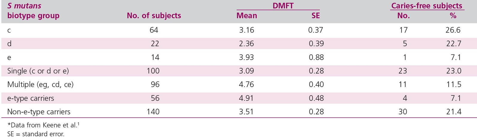
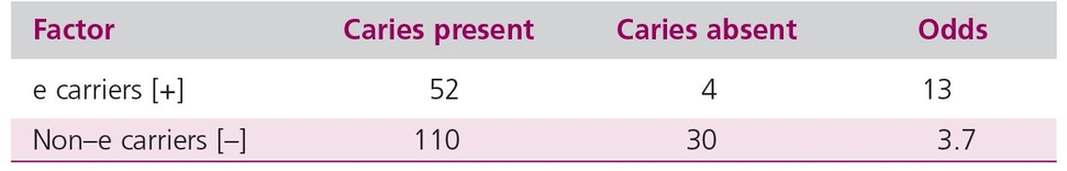
Table 17-2 Odds for caries using data from Table 17-1
Statistical considerations and calculations
Correlational studies have statistical considerations. The groups formed from exposure and outcome (eg, caries-free individuals exposed to e-biotype S mutans) could end up with very different sample sizes, and statistical efficiency could be poor. Various calculations, such as the odds ratio, can demonstrate the presence or absence of a relationship between the two variables under study (in our example, caries and S mutans biotype). Some calculations may be better than others. The criticism of statistical tests used in correlation involves methods outside the scope of this book; detailed information is presented elsewhere.3456 However, two simple statistical approaches are given here: the odds ratio and the contingency table analysis using the Cohen Kappa.
Odds ratio
The odds ratio is a widely used means that can show the relationship between factors and disease. Odds are defined as the ratio that something is so, or will occur, to the probability that it is not so, or will not occur. In looking at the odds, we could express the data in Table 17-1 in a different way (Table 17-2). For e-type carriers, the odds of having caries are 52/4 = 13. For non-e-type carriers, the odds are 110/30 = 3.7. The odds ratio—the ratio of one odds to another—is 13/3.7. An odds ratio of 1 means there is no association between the factor and the disease. Here, the odds ratio is greater than 1, and there is an association between having S mutans e-type and the disease.
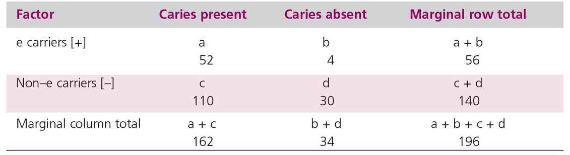
The Cohen Kappa
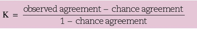
In the view of Norman and Streiner,7 the best measure of association for a contingency table with an equal number of rows and columns is the Cohen Kappa. It is defined as:
The data on caries presence or absence in relation to e-biotype can be extracted from Table 17-1 in the form of a contingency table (Table 17-3) (see also chapter 14).
The Cohen Kappa concentrates on the diagonal cells. That is, the upper left cell, a (positive for caries and positive for e-type), would be expected to have a high frequency if there were a strong association between e-type and caries, as would the lower right cell, d (absence of e-type and absence of disease). If there were a perfect association, all the cases would be found only in those two quadrants. However, in Keene et al’s data,2 the sum of quadrant a (52) with quadrant d (30) divided by the grand total (196) is 0.42 of the sample; this is the observed agreement for the association. If there were no association between e-type and caries, the individuals would be distributed into the four cells by chance, and the number in each cell could be determined by using the marginal totals as follows:
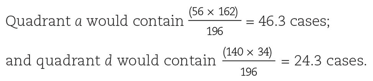
Table 17-3 Contingency table using data from Table 17-1
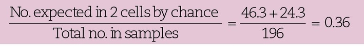
The proportion of cases expected to be distributed into the a and d quadrants by chance is thus:
Therefore, for these data:
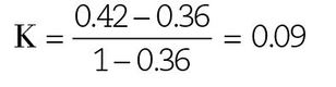
For a perfect association, K = 1, and for no association, K = 0. Thus, the association between e-type and the presence of caries is weak.
Interpretation of correlation
Authors can interpret correlation to predict future events. In our example, if the next Saudi naval recruit we saw was a carrier of the e-biotype S mutans, we might predict on the basis of the data in Table 17-1 that the recruit’s DMFT index might be higher than that of a non–e carrier. This is a legitimate use of the data. A second, and less conservative, use of the data would be to assert that the e-biotype S mutans is more effective than other serotypes in causing caries. The data are compatible with such a proposal, but the authors carefully avoid asserting it. Instead, they state, “it will be most interesting to determine whether these relationships can be demonstrated under carefully controlled laboratory conditions in the animal model.”2
The reason for their caution is the fallacy of concomitant variation, which is the fallacy of assuming that Mill’s principle of concomitant variation is necessarily true. While it is possible that two events showing a high incidence of correlation are causally connected, it is not always the case. For example, Huff8 states that there is a close relationship between the salaries of Presbyterian ministers in Massachusetts and the price of rum in Havana. However, there is no reason to suspect that the one influences the other. Thus, when applying the principle of concomitant variation, we must remember Hume’s second criterion for causation (see chapter 7): There must be some plausible reason explaining cause and effect.
Another problem with correlational studies is the linked or confounding variable (or confounder). Sometimes, when varying one condition, an investigator also varies another factor, either knowingly or unknowingly. The hoary example used to illustrate this problem relates the story of a philosopher who started out drinking scotch and soda at a party. When the host ran out of scotch, the philosopher switched to rye and soda, and finally to bourbon and soda. Carefully selecting the best correlation, the philosopher concluded that soda water was the cause of his intoxication. This example illustrates the common problem of a confounder producing an apparent association (drunkenness and soda) where none actually exists, but confounders can also diminish, reverse, or exaggerate an apparent association.
The effect of any confounder can be important only if its association with the effect of interest is strong. The most common strategy used by epidemiologists to eliminate confounders begins with consideration of possible confounding variables that might be associated with the independent variable of interest. A number of variables that are often relevant to epidemiologic studies would be investigated, including sex, parity, ethnic group, religion, marital status, social class, education, occupation, rural or urban residence, and geographic mobility. The investigator then regroups the data to see if the possible confounder has any effect on the association. A study on the prevalence of root caries for individuals living in an extended-care facility might show that caries was more prevalent in women than men. However, subsequent analysis might demonstrate that the association was modified by the sample containing more elderly women than men (because women live longer) and that prevalence of root caries was related to age, not sex.
Investigators generally accept that the best way to elucidate causation is to vary experiment factors separately, and scientists are skeptical when surveys are substituted for experiments. In a survey, investigators try to define their groups precisely, but it is always possible that two variables will be confounded and that an investigator will attribute the effect to the wrong cause. In the example of the drunken philosopher, the linked variables were alcohol (the hidden variable) and soda.
A second difficulty arises because all the data are collected at a single point in time. This leads to problems in interpreting cause-effect relatio/>
Stay updated, free dental videos. Join our Telegram channel
VIDEdental - Online dental courses


