Introduction
In this study, we aimed to verify whether different levels of maxillary incisal edges influence the perception of smile attractiveness and whether gingival display affects this perception according to groups of orthodontists, dentists, orthodontic patients, and laypersons.
Methods
Photographs of the smiles of 1 man and 1 woman showing the gingival contours of the incisors and the canines were digitally altered, creating steps from 0 to 2.0 mm in 0.5-mm increments, with and without gingival exposure. The 20 pictures were shown in random order to 240 evaluators divided into 4 groups who were asked to provide attractiveness scores on visual analog scales.
Results
Both the steps ( P <0.001) and the gingival exposure ( P <0.05) had statistically significant influences on the evaluations in all groups. There was also a statistically significant difference ( P <0.001) between the evaluations of orthodontists and the other groups, with distinct patterns.
Conclusions
The most accepted vertical relationship of incisor borders was the 1.0-mm step. There were significant differences in the evaluation of orthodontists when compared with the other 3 groups, and no significant difference was detected between these groups. The gingival display altered significantly the esthetic perception of the smiles evaluated. There were significant differences between the evaluations of the smiles of the man and the woman.
Highlights
- •
The 1.0-mm step was preferred among all groups.
- •
Extreme steps (0 and 2 mm) were equally rejected in all groups.
- •
Gingival exposure has a positive impact on smile attractiveness.
- •
Orthodontists are more strict and less tolerant to deviations than other groups.
- •
Dentists prefer smiles with more dominant central incisors.
Because of its subjective nature, it is hard to measure the beauty of a smile. However, orthodontists require tangible references regarding the factors that comprise harmonic smiles to identify their deviations and elaborate evidence-based treatment plans to create attractive smiles.
Orthodontic planning should be based on the esthetic demands of the patient, in contrast to function-driven treatment plans that create functionally perfect, although not necessarily esthetic, smiles.
An adequate smile arch, with incisors aligned in a curve parallel to the lower lip contour, is an important factor in the construction of an attractive smile. The vertical position of the incisors is of paramount importance in the formation of a more pleasant smile. Straight or reversed smile lines have already been considered to be less attractive by many authors, whereas more convex lines are considered more beautiful and youthful.
With that in mind, a great uncertainty about the best vertical relationship between the lateral and central incisor borders for each patient emerges during the planning, bonding, and finishing procedures. The orthodontist’s concepts of what is more attractive do not always coincide with the patient’s or the referring clinician’s expectations, even though some studies suggest that there is no difference among evaluator groups.
For that reason, it is important to address the relationship of the incisal borders for a more esthetic smile, among not only orthodontic patients and orthodontists but also dentists and laypersons. In this way, orthodontists may have a reference to support the communication with those groups, helping to achieve common treatment goals.
Considering these issues, in this study we aimed to determine (1) the most accepted vertical relationship of incisor borders, (2) whether there is a difference in the esthetic perceptions among different groups of evaluators, (3) whether gingival display alters this perception, and (4) whether there are differences between the evaluations of the smiles of men and women.
Material and methods
This project was approved by the research ethics committee of Universidade Federal Fluminense, Niterói, Rio de Janeiro, Brazil (number 643.906).
The photographs of smiles of 2 volunteers—a man and a woman—showing the gingival contours of the maxillary teeth had 1 side digitally altered with Adobe Photoshop (version CS5; Adobe Systems, San Jose, Calif) to adjust the proportion of the teeth according to the literature. Distractions, such as color, shape, and size alterations, of the teeth and surrounding structures were removed. The volunteers signed a release form for use of their images for scientific research by the Department of Orthodontics of the university.
The new manipulation simulated changes to the vertical relationship of the incisor borders, varying from 0.0 to 2.0 mm in 0.5-mm steps exclusively by extrusion of the central incisors. No alterations were made to the crown length or the height-width ratio of the incisors.
To precisely graduate the vertical movement, the real incisors of the volunteers were measured with a digital caliper (Lotus, Serra, Espirito Santo, Brazil). A virtual ruler was then calibrated in proportion to the measurement in the software to standardize the 0.5-mm increments.
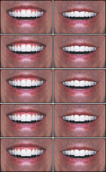
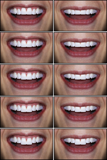
We made another manipulation, which consisted of downward movement of the upper lip so that all gingival contours of the canines and the incisors were hidden on the 2.0-mm extrusion of the central incisors. The side that was manipulated was then mirrored to ensure perfect symmetry. All manipulations were made by the same operator (R.M.M.) and resulted in 20 images, 10 for each sex ( Figs 1 and 2 ).
The sample size was calculated with G*Power software (version 3.1.9.213; Heinrich Heine Universitat Dusseldorf Institute Experimentelle Psychologie, Dusseldorf, Germany), considering an alpha error of 0.01, 80% power, and 0.25 effect size. The total sample size suggested was 239 subjects. Then, 60 evaluators were recruited in each of 4 groups (orthodontists, dentists, orthodontic patients, and laypersons), resulting in 240 evaluators. This number was consistent with studies that used similar methods.
As inclusion criteria, the evaluators were required to be between 18 and 60 years old, with no sex distinction. Participants in the orthodontic patients group were required be involved in active orthodontic treatment for at least 6 months in private offices or at the clinic of the Department of Orthodontics at the university. Those in the layperson group were required to have a completed or an uncompleted college degree. They were randomly selected from among students in graduate courses at the university, unrelated to dentistry. The members of the dentist group were required to have graduated more than 2 years previously and to practice any specialty other than orthodontics. The group of orthodontists included specialists who worked with fixed orthodontics techniques.
Dentists, dental students, and spouses of dentists were excluded from the layperson and orthodontic patient groups. All volunteers provided informed consent.
To grade smile attractiveness, a sheet with 20 visual analog scales (VAS) 100 mm wide was used, with zero (0 mm) as the most unattractive and 100 (100 mm) as the most attractive. The measurements were made with the same digital caliper by the same operator (R.M.M.).
Using Keynote software (version 6.1; Apple, Cupertino, Calif), the 10 manipulated pictures of each model were assembled in a presentation. After a brief explanation of the study and how to use the VAS, a slide with all pictures of the male model’s smile in increasing order of incisal steps was displayed for 20 seconds as a calibration method. After that, the same 10 pictures were shown, one by one, in random order. The transition was automatic after 15 seconds of display. The same procedure was then repeated for the smiles of the woman. The pictures were shown on either a tablet or a computer screen for luminosity control. Reevaluation of the pictures was not allowed.
The exact wording given to the evaluators was this: “Please give grades to the following pictures according to their attractiveness, considering 0 as extremely unattractive and 10 as extremely attractive. The grades can be marked at any point of the scale, as shown in the example. The transition of pictures is automatic. There will be 10 pictures of each person, which will be displayed, at first all together for 20 seconds, and then in random order, one by one, for 15 seconds each. The grading must be done when they are displayed one by one. It is not allowed to reevaluate the pictures.” The evaluators were not told at any point which characteristics would be altered in the pictures.
To compensate for printing distortions on the VAS sheet, the first VAS of each page was measured, and each score was adjusted proportionally.
Statistical analysis
Statistical analysis was made with software (version 20; IBM, Armonk, NY). The normality of the sample was checked with Shapiro-Wilk and Kolmogorov-Smirnov tests. Descriptive statistics used frequencies, means, standard deviations, maximums, and minimums ( Table I ).
| Group | n | Sex | Age (y) | |||
|---|---|---|---|---|---|---|
| Male | Female | Mean | Minimum | Maximum | ||
| Orthodontists | 60 | 20 | 40 | 37.82 ± 08.67 | 25 | 58 |
| Dentists | 60 | 20 | 40 | 37.98 ± 06.21 | 29 | 55 |
| Patients | 60 | 17 | 43 | 30.85 ± 07.95 | 20 | 55 |
| Laypersons | 60 | 14 | 46 | 29.12 ± 12.83 | 18 | 59 |
| Total | 240 | 71 | 169 | 33.94 ± 10.02 | 18 | 59 |
Repeated-measures analysis of variance (SPANOVA) with the Tukey post hoc test at a 5% significance level was conducted, considering 1 between-groups (evaluator group) and 3 within-subjects (smile model sex, incisal step, and gingival contour exposure) factors. To determine the effect size (partial eta squared) and the significance level of the SPANOVA, the Greenhouse-Geisser test was performed. The Huynd-Feldt correction was applied to adjust the degrees of freedom of the F tests, and therefore the P value wherever there was violation in the sphericity on Mauchly’s test. This was also 1 more action to control the tendency of increase in the type I error during the comparisons.
These analyses verified not only the isolated influence of each factor but also the effect of its interactions. The partial eta squared results for each factor or interaction show the proportional quantification of its participation on the esthetic perception, excluding the other factors.
Three judges from each group were asked to reevaluate the 20 photographs at least 2 months after the first test. A correlation test was taken, and a coefficient of 0.833 (83.3%; 95% confidence interval, 0.782-0.872) was found, ensuring reliability.
Results
The sample was composed of 240 evaluators ( Table I ), 29.6% men and 70.4% women.
The means for each picture, grouped and divided by the evaluator group, are shown in Table II . The highest ranked pictures without gingival exposure were the 1.0-mm step for both sexes. For the pictures with gingival exposure, the 0.0-mm step for the smile of the man and the 0.5-mm step for the smile of the woman received the highest grades.
| Picture | Orthodontists | Dentists | Patients | Laypersons | Total |
|---|---|---|---|---|---|
| MN00 | 57.06 ± 18.28 | 64.58 ± 15.85 | 71.57 ± 16.68 | 69.19 ± 16.16 | 65.60 ± 17.56 |
| MN05 | 55.30 ± 20.24 | 65.59 ± 14.72 | 73.81 ± 14.48 | 70.41 ± 15.01 | 66.27 ± 17.57 |
| MN10 | 67.72 ± 17.82 | 68.34 ± 18.67 | 73.60 ± 15.13 | 68.90 ± 17.72 | 69.64 ± 17.43 |
| MN15 | 64.65 ± 17.50 | 70.30 ± 13.98 | 71.56 ± 16.22 | 70.43 ± 14.22 | 69.24 ± 15.69 |
| MN20 | 61.11 ± 18.81 | 70.50 ± 14.52 | 69.61 ± 17.20 | 66.23 ± 17.96 | 66.86 ± 17.48 |
| ME00 | 65.26 ± 15.37 | 69.85 ± 16.32 | 73.70 ± 17.22 | 75.87 ± 14.95 | 71.17 ± 16.40 |
| ME05 | 64.55 ± 15.83 | 67.47 ± 13.34 | 75.50 ± 14.75 | 70.79 ± 14.96 | 69.57 ± 15.20 |
| ME10 | 68.05 ± 19.13 | 67.45 ± 16.06 | 76.19 ± 14.54 | 68.28 ± 17.20 | 69.99 ± 17.09 |
| ME15 | 67.08 ± 19.93 | 68.60 ± 15.04 | 69.92 ± 16.45 | 72.09 ± 14.33 | 69.42 ± 16.58 |
| ME20 | 56.61 ± 18.84 | 66.06 ± 14.73 | 67.45 ± 17.93 | 69.89 ± 14.39 | 65.00 ± 17.02 |
| FN00 | 40.10 ± 16.76 | 53.61 ± 15.13 | 61.37 ± 22.43 | 58.16 ± 19.41 | 53.31 ± 20.23 |
| FN05 | 53.18 ± 15.38 | 61.23 ± 16.42 | 68.62 ± 18.38 | 60.38 ± 18.89 | 60.85 ± 18.07 |
| FN10 | 68.94 ± 17.39 | 78.03 ± 12.99 | 77.01 ± 14.32 | 71.11 ± 17.21 | 73.77 ± 15.97 |
| FN15 | 56.10 ± 12.12 | 68.27 ± 13.80 | 66.12 ± 19.20 | 62.69 ± 16.94 | 63.30 ± 16.33 |
| FN20 | 52.56 ± 16.61 | 66.73 ± 15.71 | 63.55 ± 22.84 | 61.53 ± 18.25 | 61.09 ± 19.18 |
| FE00 | 50.95 ± 17.25 | 61.69 ± 16.59 | 72.70 ± 17.50 | 62.56 ± 19.96 | 61.98 ± 19.36 |
| FE05 | 73.85 ± 13.48 | 75.47 ± 12.67 | 84.01 ± 14.77 | 75.58 ± 16.41 | 77.23 ± 14.86 |
| FE10 | 74.07 ± 12.95 | 77.00 ± 12.82 | 79.42 ± 15.37 | 72.60 ± 14.97 | 75.78 ± 14.23 |
| FE15 | 57.37 ± 14.55 | 66.36 ± 13.25 | 63.52 ± 20.23 | 61.62 ± 18.30 | 62.22 ± 17.03 |
| FE20 | 42.57 ± 14.40 | 57.76 ± 16.50 | 56.03 ± 24.90 | 56.28 ± 18.12 | 53.16 ± 19.76 |
The estimated marginal means of the SPANOVA allowed for the evaluation of each factor, eliminating the interference of the others. A great reduction in the standard deviation was observed. This occurred because in the descriptive statistics, the means referred to 1 picture, which was a combination of all factors analyzed by the 240 evaluators, producing a mean of 240 scores.
On the other hand, when an isolated factor was evaluated, this mean would be the result of all possible combinations of that factor. For instance, if we considered the incisal step alone, it would receive scores for each of the 240 evaluators in each of the 2 gingival exposure possibilities in each of the 2 sex variations. The total number of scores composing this mean would be 240 × 2 × 2 = 960. Because the number of scores was significantly higher, the standard deviation would be much smaller, and since it originated from different scores, the step with the higher score may be different from the one of the highest ranked picture. This logic can be applied to all of the studied factors.
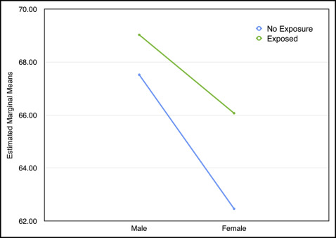
The graphic representations of the variations on the estimated marginal means, when crossing group vs step, gingival exposure vs step, sex vs step, gingival exposure vs groups, and gingival exposure vs sex, whether statistically significant or not, can be seen in Figures 3 to 7 .
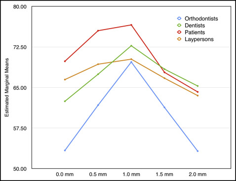
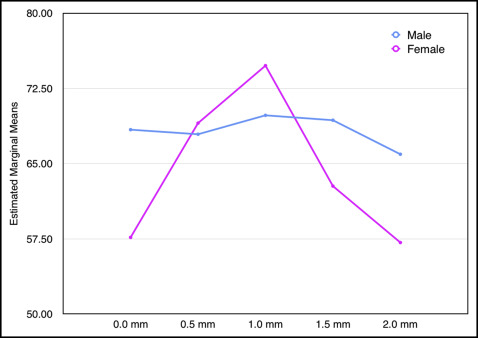
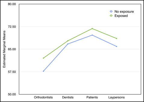

The variations of all studied factors (evaluator group, incisal step, gingival exposure, and sex) showed statistically significant differences when isolated. The interactions of 2 or more factors did not show statistically significant differences in all situations. The quantification of this effect is indicated by the partial eta squared results (effect size), and the more relevant observations were associated with the incisal step ( Table III ). The results of the SPANOVA are presented in Table IV .
| Source | P | Partial eta squared ∗ |
|---|---|---|
| Sex | 0.000 † | 0.115 |
| Sex + group | 0.066 | 0.030 |
| Gingival exposure | 0.000 † | 0.062 |
| Gingival exposure + group | 0.336 NS | 0.014 |
| Step | 0.000 † | 0.289 |
| Step + group | 0.000 † | 0.107 |
| Sex + gingival exposure | 0.009 † | 0.029 |
| Sex + gingival exposure + group | 0.683 NS | 0.006 |
| Sex + step | 0.000 † | 0.284 |
| Sex + step + group | 0.000 † | 0.039 |
| Gingival exposure + step | 0.000 † | 0.271 |
| Gingival exposure + step + group | 0.000 † | 0.039 |
| Sex + gingival exposure + step | 0.000 † | 0.139 |
| Sex + gingival exposure + step + group | 0.186 NS | 0.017 |
∗ Correspondent to effect size; † statistically significant ( P <0.05).
| Group | Mean difference | SD | P ∗ |
|---|---|---|---|
| Orthodontists | |||
| Dentists | −7.390 ∗ | 1.959 | 0.001 |
| Patients | −10.911 ∗ | 1.959 | 0.000 |
| Laypersons | −7.375 ∗ | 1.959 | 0.001 |
| Dentists | |||
| Patients | −3.522 | 1.959 | 0.277 |
| Laypersons | 0.015 | 1.959 | 1.000 |
| Patients | |||
| Laypersons | 3.536 | 1.959 | 0.273 |
∗ Significant at P <0.050 (Bonferroni correction for multiple comparisons).
Results
The sample was composed of 240 evaluators ( Table I ), 29.6% men and 70.4% women.
The means for each picture, grouped and divided by the evaluator group, are shown in Table II . The highest ranked pictures without gingival exposure were the 1.0-mm step for both sexes. For the pictures with gingival exposure, the 0.0-mm step for the smile of the man and the 0.5-mm step for the smile of the woman received the highest grades.


