In statistics, we use a random sample from the population of interest to draw conclusions and make inferences about the population. If the sample does not represent the population of interest, then inferences from data derived from the sample might not be valid. For example, determining the effect of an intervention for adolescents based on the results from a sample of adults could yield the wrong conclusion.
The sampling distribution
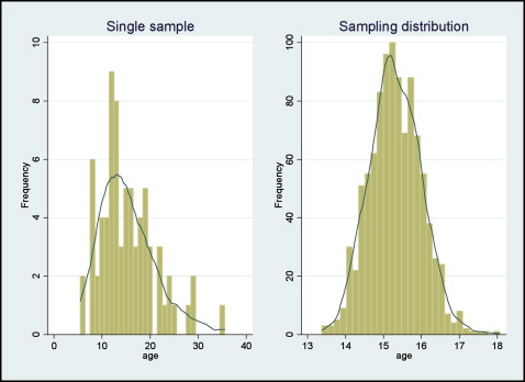
The first of the 2 plots ( left ) in Figure 1 shows the distribution of age from 1 sample drawn from a population of interest. We can see some skewness in the data; however, no gross deviations from normality are observed. The right plot with normally distributed data is the distribution of the means from 1000 random samples drawn from the same population of interest as the left plot. The distribution of the sample means on the right is called the sampling distribution. The sampling distribution is the distribution of all possible sample means that could be drawn from the population, but it is almost always a hypothetical distribution because typically we cannot calculate every conceivable sample mean. The mean of the sampling distribution is an unbiased estimator of the population mean with a computable standard deviation. The notion of the unbiased estimator is based on the idea that if samples of the same size are repeatedly extracted from a population and their mean values are calculated with the common formula, then on average these mean values will approach the population mean.
The interesting part is that the sampling distribution (distribution of the means) regardless of the distribution of the single-sample data from the target population follows a normal distribution, and this characteristic is used to make statistical inferences.
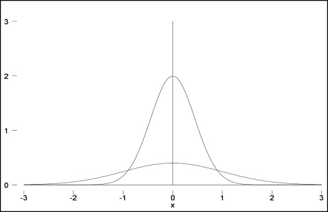
As the sample size increases, the margin of error gets smaller: ie, the sampling distribution is more peaked, and the estimate is more precise. The sampling distribution plot in Figure 2 shows 2 curves ( wide and narrow ) that have the same mean but different numbers of samples. The wide sampling distribution includes only 1 sample, whereas the narrow sampling distribution includes 25 samples. As the number of samples increases, the spread of the distribution becomes more narrow; hence, the precision (width around the mean) increases.