Introduction
The purpose of this study was to determine, by statistical shape analysis of original and mirrored skeletal landmarks, the optimal landmark-based midsagittal reference plane for evaluation of facial asymmetry.
Methods
The study sample comprised 69 patients with facial asymmetry (36 men, 33 women; mean age, 23.0 ± 4.1 years). All landmarks were obtained with cone-beam computed tomography using a 3-dimensional coordinate system. For identifying the landmark-based midsagittal reference plane, the 3 landmarks nearest to the symmetric midsagittal reference plane were selected by ordinary and generalized Procrustes analyses. To verify the 3-landmark-based midsagittal reference plane’s compatibility with the symmetric midsagittal reference plane, asymmetry measurements were calculated and tested for each.
Results
The 3 nearest landmarks (nasion, anterior nasal spine, and posterior nasal spine) were selected for the 3-landmark-based midsagittal reference plane. The averages of the sums of the squared Euclidean distance and the squared Procrustes distance differences between the 2 configurations and shapes fabricated by the symmetric and landmark-based midsagittal reference planes, respectively, were calculated as 0.121 ± 0.241 mm and 1.69 × 10 −6 ± 3.25 × 10 −6 . The testing results for the symmetric and landmark-based midsagittal reference planes were almost the same.
Conclusion
The results indicated that a 3-dimensional midsagittal reference plane constructed of nasion, anterior nasal spine, and posterior nasal spine could be a valuable tool for the evaluation of patients with facial asymmetry.
Highlights
- •
We proposed a midsagittal reference plane to evaluate facial asymmetry.
- •
The proposed plane is the landmark-based midsagittal reference plane.
- •
Statistical shape analysis determines the landmarks constituting the plane.
- •
The landmarks are nasion, anterior nasal spine, and posterior nasal spine.
- •
This plane was compatible with a symmetric midsagittal plane.
In the past, most patients with facial asymmetry who underwent orthognathic surgery had severe maxillofacial deformities, but lately, amid improved socioeconomic conditions and with the increased interest in appearance, many people are eager to correct even a slight facial asymmetry. The need for accurate analysis of facial asymmetry has increased concomitantly and now includes the factors that directly contribute to asymmetry and determine its treatment. Unfortunately, a perfectly symmetric face is rare. Bilateral landmarks tend to show the asymmetric positions from the skull base to the chin area. This means that reference planes constructed with such craniofacial structural landmarks could be used for a uniquely effective assessment of facial asymmetry. The reference plane setup, therefore, is the most important step in treatment planning for facial asymmetry.
Most studies on facial asymmetry have been based on 2-dimensional imaging methods such as clinical photography and posteroanterior cephalography. These methods, however, cannot account for the 3-dimensional (3D) nature of the face. In response to this problem, various 3D imaging techniques have been developed. Hwang et al proposed a facial asymmetry analysis method that uses computed tomography and offers, as reference planes, the Frankfort horizontal plane and the midsagittal plane composed of 3 landmarks: opisthion, crista galli, and anterior nasal spine (ANS). Hajeer et al established an alternative, soft-tissue reference plane using an individual symmetric configuration that was computed according to the average of the original and mirror images in 3D stereophotogrammetry. They used that reference plane to assess facial asymmetry before and after orthognathic surgery. Wong et al proposed, for evaluation of facial asymmetry, a voxel-based matching optimal symmetry plane method that automatically overlaps with an optimized algorithm and can set up a midsagittal plane without a landmark.
For effective correction of facial asymmetry, accurate evaluation is essential, for which it is necessary to set up the midsagittal reference plane. Previous studies, for the purposes of accurate analysis, determined the reference plane with superimposition between the original and mirror images. These reference planes were individualized without specific cephalometric landmarks. However, cephalometric landmark-based reference planes should be easier to use and, thus, preferable to orthodontic practitioners. The aim of this study, therefore, was to find, using ordinary Procrustes analysis from original and mirror skeletal landmarks, the optimal landmark-based midsagittal reference plane for evaluation of facial asymmetry. Our specific aims were (1) to establish the symmetric midsagittal reference plane from the bilateral skeletal landmarks of the original shape and its mirrored shape with the ordinary Procrustes analysis superimposition method, and (2) to propose a clinically useful landmark-based midsagittal reference plane composed of the existing cephalometric landmarks nearest to the symmetric midsagittal reference plane.
Material and methods
This was a retrospective study. The study group comprised 69 patients with facial asymmetry (36 men, 33 women; mean ages: women, 23.0 ± 4.2 years; men, 22.9 ± 4.1 years; total, 23.0 ± 4.1 years) undergoing treatment at the Department of Orthodontics, Pusan National University Dental Hospital, Yangsan, South Korea. The Angle classifications of patients were as follows: Class I, 10 patients; Class II, 12 patients; Class III, 47 patients ( Table I ). All had a mildly to moderately deviated menton (mean deviation, 3.6 ± 2.3 mm) on posteroanterior cephalography regardless of the Angle classification. The exclusion criteria were cleft lip or palate, craniofacial syndrome, and facial trauma. This study was reviewed and approved by the institutional review board of Pusan National University Dental Hospital (PNUDH-2015-003).
| Class I (n = 10) | Class II (n = 12) | Class III (n = 47) | P value | |
|---|---|---|---|---|
| Sex (female/male) | 6/4 | 7/5 | 23/24 | 0.524 |
| Age (y) | 21.23 ± 3.35 | 24.25 ± 3.41 | 23.18 ± 4.14 | 0.217 |
| SNA (°) | 80.26 ± 2.25 | 81.84 ± 2.60 | 80.02 ± 2.60 | 0.108 |
| SNB (°) | 79.16 ± 2.32 a | 77.81 ± 2.93 a | 82.86 ± 3.14 b | 0.000 |
| ANB (°) | 1.11 ± 0.45 a | 4.02 ± 1.34 b | -2.84 ± 2.06 c | 0.000 |
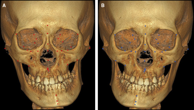
The landmarks were acquired from cone-beam computed tomography (CBCT) images. The skeletal landmarks were obtained on 3D CBCT images. The CBCT scanner (Zenith3D; Vatech, Seoul, Korea) was set to a 90-kVp tube voltage, a 4-mA tube current, 0.3-mm voxel size, and a 24-second scan time, with the Frankfort horizontal plane parallel to the floor. The CBCT data thus acquired were processed in 3D x-, y-, z-coordinate images by Ondemand3D software (Cybermed, Seoul, Korea).
The axes were defined as follows. The x-axis, determined first, included nasion (Na) and ran between the right and left orbitales. The y-axis included Na and ran perpendicular to the x-axis on the Frankfort horizontal plane. The z-axis included Na and ran perpendicular to the x-axis and y-axis. The common origin (0, 0, 0) of the 3 axes was Na.
The landmarks were as follows ( Table II ). The bilateral landmarks were the foramen ovale, foramen rotundum, foramen spinosum, hypoglossal canal, internal acoustic meatus, jugular foramen, orbitale, infraorbitale, supraorbitale, porion, and greater palatine canal, as well as the most inferior points of the frontozygomatic and zygomaticomaxillary sutures. The landmarks on the midline were Na, sella, basion, opisthion, A-point, anterior nasal spine (ANS), posterior nasal spine (PNS), and nasopalatine canal. All landmark positions were recorded in their x, y, z coordinates.
| Landmark | Definition |
|---|---|
| Bilateral landmarks (right and left) | |
| Foramen ovale | Center of the foramen ovale |
| Foramen rotundum | Center of the foramen rotundum |
| Foramen spinosum | Center of the foramen spinosum |
| Frontozygomatic suture | Medial point of the orbital rim of the zygomaticofrontal suture |
| Greater palatine canal | Center of the opening of the greater palatine canal |
| Hypoglossal canal | Center of the right hypoglossal canal |
| Infraorbitale | Center of the opening of the greater palatine canal |
| Orbitale | Lowest point in the inferior margin of the orbit |
| Porion | Superior point of the upper contour of the external auditory meatus |
| Supraorbitale | Center of the supraorbital foramen |
| Zygomaticomaxillary suture | Superior medial point of the zygomaticomaxillary suture |
| Landmarks on midline structure | |
| A-point | Deepest point on the innermost curvature from the maxillary ANS to the crest of the maxillary alveolar process |
| ANS | Tip of the bony ANS |
| Basion | Mid-dorsal point of the anterior margin of the foramen magnum |
| Inferior nasopalatine canal | Most inferior point of the posterior border of the nasopalatine canal |
| Nasion | Most anterior point of the frontonasal suture on the median plane |
| Nasopalatine canal | Lowest point of the opening of the nasopalatine canal |
| Opisthion | Middle point on the posterior margin of the foramen magnum, opposite the basion |
| PNS | Tip of the bony PNS |
| Sella | Center of the hypophyseal fossa (sella turcica) |
| B-point | Deepest point between the chin and the mandibular incisors |
| Menton | Most inferior point on the chin in the lateral view |
| Genial tubercle | Most posterior point of the genial tubercle |
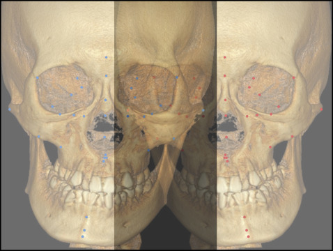
The individual symmetric midsagittal reference planes were each generated in the following steps ( Figs 1-3 ): (1) establishing the center of the original configuration as the origin, (2) obtaining the mirrored configuration from the original configuration around the YZ plane, (3) superimposing the original on its mirrored configuration and the mirrored on the original configuration using partial ordinary Procrustes analysis, and (4) after aligning 2 superimposed configurations called Procrustes fits, creating the individual symmetric configuration according to the arithmetic mean of those fits. The individual symmetric midsagittal reference plane was calculated on that basis.
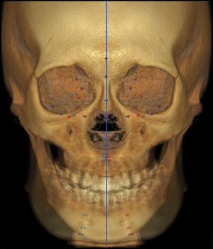
For the purpose of identifying the landmark-based symmetric midsagittal reference planes, the cephalometric landmarks on the midline structure were tested to find those at the smallest distance from the symmetric midsagittal reference plane. To measure the distances between the individual symmetric midsagittal reference plane and the landmarks on the midline structure, all original and corresponding mirrored configurations were superimposed by full generalized Procrustes analysis, and the mean values were calculated ( Table III ). The 3 landmarks with the smallest distances were then used to draw the landmarks-based symmetric midsagittal reference plane.
| Na | ANS | PNS | NPC | A-point | Opisthion | Sella | Basion | |
|---|---|---|---|---|---|---|---|---|
| Mean | 0.697 | 0.755 | 0.775 | 0.819 | 0.823 | 1.047 | 1.064 | 1.041 |
| SD | 0.542 | 0.527 | 0.723 | 0.681 | 0.570 | 0.869 | 0.999 | 1.071 |
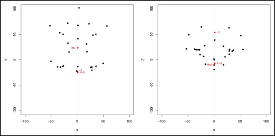
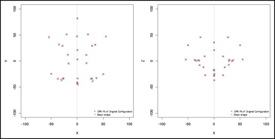
The 3-landmark-based plane’s compatibility with the individual symmetric midsagittal reference plane was verified by measuring the asymmetry for each and testing it based on the study of Mardia et al. The asymmetry of the 3-landmark-based plane was measured as follows ( Figs 4 and 5 ): (1) estimating the multiple regression line of the 3-landmark coordinates for each centered original configuration (the response variable of the regression line is the x-axis coordinate), (2) obtaining X i for i = 1, …, n , which is the configuration of rotating the original configuration as the estimated regression line is perpendicular to the x-axis, (3) determining the mirrored configuration Y i from the rotated configuration X i around the YZ plane, (4) calculating the individual symmetric configurations S i of the Procrustes fits by the interactive ordinary Procrustes analysis of the X i and Y i , and (5) measuring the asymmetry for each configuration as follows (see the Supplemental Material for more details).
Let X i for i = 1, …, n be the i th configuration, and let S i be the individual symmetric configuration of X i and the mirrored configuration Y i of X i . Then the sum of the squared Euclidean distances is defined as the sum of distances between the corresponding landmarks of X i and S i . However, the sum of the squared Euclidean distances depends on location, scale, and rotational effects of X i . So, we consider another measure to analyze asymmetry, the squared Procrustes distances of the shapes. Here, “shape” means all the geometric information that remains when location, scale, and rotational effects are filtered out from a configuration. Therefore, first we must obtain a centered configuration from X i . Then to remove the scale effect from X i , we divide the centered configuration to the centroid size of X i , and we call it the centered preshape. Since the location and scale effects are filtered out, all centered preshapes have the same scale. Then the squared Procrustes distances can be obtained by matching the centered preshape of X i for i = 1,…, n and that of S i as closely possible over rotations. It can be obtained by the ordinary Procrustes analysis solution. Hence, the squared Procrustes distance is a measure for the asymmetry that does not depend on location, scale, and rotational effects of the original configuration, X i .
Based on the same manner as the sum of the squared Euclidean distances and the squared Procrustes distances, the amount of asymmetry was calculated as follows: (1) by comparing landmark changes between the original and symmetric configurations and shapes for the 2 methods, respectively; and (2) by comparing the differences of the amount of asymmetry between the 2 configurations and 2 shapes produced by the 2 methods.
We compared the total variations for asymmetry measurements according to 2 (symmetric and 3-landmark-based) midsagittal reference planes. Mardia et al proposed an object-symmetry testing procedure that uses the close approximation of the Euclidean metric in the tangent space to the true Procrustes distance. In this way, Procrustes tangent projections XPi
X i P
and YPi
Y i P
can be obtained from Procrustes fits by the generalized Procrustes analysis of X i and Y i with respect to the full Procrustes mean shape ˉG
G ¯
. The Procrustes tangent projections XPi
X i P
and YPi
Y i P
have the same meaning as the centered preshapes, and ˉG
G ¯
is symmetric and has the same shape as the ordinary average 12(ˉXP+ˉYP)
1 2 ( X ¯ P + Y ¯ P )
, where ˉXP
X ¯ P
and ˉYP
Y ¯ P
are the arithmetic means of XPi
X i P
and YPi
Y i P
, respectively. Accordingly, it is possible to decompose the asymmetry of all data as follows (see the Supplemental Material for more details).
The total variations for the asymmetry of all data are defined as the sum of squares of the distances between the corresponding landmarks of XPi
X i P
and YPi
Y i P
. The total variation of the asymmetry SS T can be decomposed as the variations between mean shapes and the variations within subjects. The variation between mean shapes is defined as the sum of squares of the distances between the corresponding landmarks of ˉXP
X ¯ P
and Y ¯ P
Y ¯ P
; it means the between-squares side, SS B , for asymmetry. The variations within subjects can be measured by the sum of squares of the distances between the corresponding landmarks of X i P − X ¯ P
X i P − X ¯ P
and Y i P − Y ¯ P
Y i P − Y ¯ P
; the variations can be denoted by the within-subjects sum of squares, SS W . Using this method, it is possible to test the asymmetry of the population in the same manner as 1-way analysis of variance (ANOVA).
All landmarks were remeasured at 2-week intervals by 2 investigators (S.M.S., Y-M.K.). The systematic intraexaminer and interexaminer errors between the 2 measurements were determined with a paired t test. Also, the magnitudes of those errors were assessed by calculating the intraclass correlation coefficient (ICC). For statistical computation purposes, the language R (Vienna, Austria) was used.
Stay updated, free dental videos. Join our Telegram channel
VIDEdental - Online dental courses


