In previous statistical articles, we demonstrated how to use multilevel linear or nonlinear models to analyze longitudinal orthodontic growth data. Here, we will explain how to use latent growth curve models for data with repeated measurements. From a statistical perspective, latent growth curve models and multilevel models for longitudinal data analysis are actually equivalent. However, because these 2 methods have been implemented in software packages in a different manner, they have their own advantages and limitations in practical data analyses.
Multilevel models are most useful when the number of repeated measurements is large and these measurements have been undertaken at different times for different subjects. Current software packages for latent growth curve models do not provide the same level of flexibility in coping with different time intervals between measurements among subjects. Latent growth curve models and multilevel modeling are equally useful, when (1) the repeated measurements were undertaken at the same intervals for all subjects, and (2) the number of repeated measurements is limited. When the number of repeated measurements is limited but the outcome shows a nonlinear change pattern, latent growth curve models can be a better choice. This scenario usually occurs when interventions are given to the subjects at a baseline or over a period of time, such as in clinical trials.
Latent growth curve models have been popular in social and psychological sciences for analyzing experimental and observational data. For this article, we used a simple example to show how latent growth curve models can be used for analyzing orthodontic pain data. Since latent growth curve models can be viewed as a special application of structural equation models, all software packages for structural equation models can be used for latent growth curve models analysis. All of our analyses were undertaken with the software Mplus (version 7.11; Muthen & Muthen, Los Angeles, Calif).
The data consist of repeated pain measurements on a visual analog scale (VAS) for 53 patients after placement of 2 types of orthodontic appliances, A (28 subjects) and B (25 subjects), at 4 hours, 24 hours, 3 days, and 7 days. The aim of our analysis was to evaluate whether there were differences in the pain levels at baseline and the changes in pain between the 2 groups.
Statistical analysis
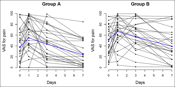
We first plotted the VAS scores for the 53 patients. Figure 1 shows individual VAS scores over 7 days for each patient in the 2 groups. For both groups, the pain levels seemed to increase with time until day 3 but slightly decreased at day 7. Table I summarizes the VAS scores on the 4 occasions for each group. Although group B showed greater levels of pain on the 4 occasions than did group A, the 2-sample t test shows that their differences were not statistically significant at the baseline (8.74; 95% confidence interval [CI], −8.34-25.82) and at 24 hours (8.67; 95% CI, −8.38-25.72), but they were significant on day 3 (20.28; 95% CI, 4.11-36.45) and day 7 (20.28; 95% CI, 4.19-34.26). When the 4 measurements of pain were summed as a total score, the differences in the total scores between the 2 groups were also statistically significant (56.91; 95% CI, 6.69-107.14). These results are statistically significant when the significance level is set at 5%. As we carried out multiple testing procedures for the same data, a more stringent significance level (such as the adjustment made by the Bonferroni correction) might be required to control the false-positive rates.
| Variable | Mean | SD | Minimum | Maximum |
|---|---|---|---|---|
| Group A (n = 28) | ||||
| 4 hours | 40.54 | 33.03 | 0 | 98.2 |
| 24 hours | 56.45 | 34.13 | 0 | 100 |
| Day 3 | 40.17 | 31.29 | 0 | 99.1 |
| Day 7 | 22.07 | 23.57 | 0 | 84.68 |
| Group B (n = 25) | ||||
| 4 hours | 49.28 | 28.35 | 5.86 | 94.59 |
| 24 hours | 65.12 | 26.72 | 4.5 | 99.55 |
| Day 3 | 60.45 | 26.82 | 1.35 | 99.55 |
| Day 7 | 41.30 | 30.82 | 0.45 | 94.59 |
For latent growth curve models, it is helpful to use a path diagram ( Fig 2 ), commonly used to portray a structural equation model, to explain the statistical concepts behind latent growth curve models. In our analysis, 4 VAS scores were made at 4 hours, 24 hours, day 3, and day 7. These 4 variables are represented by X1, X2, X3, and X4, respectively, in Figure 2 . Latent growth curve models use the 4 variables to estimate the baseline VAS and the change in VAS over the observation period by estimating first the individual baseline VAS and the change in VAS. This is exactly the same approach as multilevel models that we demonstrated previously. In multilevel models, the variations in baseline VAS are denoted as random intercepts (each patient’s baseline VAS score), whereas the variations in slopes for the changes in VAS are denoted as random slopes (each patient’s VAS score changed pattern with time); they were treated as 2 random variables in the models. In latent growth curve models, these 2 random variables are explicitly depicted as 2 latent (unobserved and to be estimated) variables, “Intercept” and “Slope.” Following the convention in structural equation models, latent variables are in circles, whereas observed variables such as VAS scores are in squares.
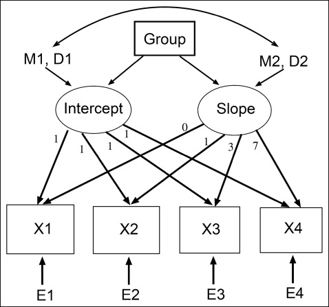
For the 2 latent variables Intercept and Slope in Figure 2 to represent the estimated intercepts and slopes, we needed to carefully set up their relationships to the 4 VAS scores; this was done by the arrows from the 2 latent variables to each X. The direction of the arrows in Figure 2 from Intercept and Slope to X and their associated factor loadings (the number next to an arrow) define their functions in the models. For instance, the relationship between VAS scores and intercept/slopes can be written as the following regression equations:
Stay updated, free dental videos. Join our Telegram channel
VIDEdental - Online dental courses


