Orthodontic research often involves collection of data on a cohort of subjects with longitudinal follow-up. For example, the study of the growth of facial profiles among boys and girls usually uses data from repeated tracings of cephalometric landmarks across childhood and adolescence. Analysis of longitudinal data is a challenging task and usually requires advanced statistical methods that might not be familiar to most orthodontic researchers. After the research questions are carefully formulated, appropriate methods are then selected according to the properties of the data, such as the number of repeated measurements for each subject, the time intervals between measurements, and the shape of the growth curves.
Several approaches are commonly used for analyzing longitudinal data.
- 1.
For changes in the outcome over a period of observation, differences in the average values between successive measurements are tested in a group of participants. The advantage of this approach is that the testing procedure is relatively straightforward, but this approach cannot take into account the variations in the subjects. Additionally, this method fails to address the changes over time in each participant, and this is usually the reason that the longitudinal design is chosen in the first place. It also invokes the problem of multiple testing that might inflate the type I error rate (the probability of false-positive results).
- 2.
For comparisons between groups, analyses are undertaken at predefined time points. This approach prespecifies the time points at which the primary comparisons will be made. For example, selected cephalometric measurements are compared between different groups at certain chronologic ages that are of particular clinical interest. Strictly speaking, this method requires the measurements of all participants to be made at the same age, and it is essentially a multiple cross-sectional analysis.
- 3.
Summary measures derived from repeated measurements for each participant and the differences in the average summary measures between groups are tested. This method reduces or eliminates the problem of multiple testing but again does not allow for the assessment of important characteristics in changes in the outcome over time.
- 4.
Statistical modeling can be used to characterize important features in the process of changes. Classical regression analyses assume that the observations are independent, but when multiple observations are collected from the same subjects, those observations are inherently correlated. So, advanced methods that can take this correlation into account must be used for longitudinal data analysis.
In this article, we will use an example to show how longitudinal orthodontic data can be analyzed using multilevel modeling (also known as hierarchical linear modeling or random effects modeling) and illustrate how multilevel modeling outperforms the aforementioned methods. Multilevel modeling was first developed to analyze clustered data in which observations were not independent, such as patients treated by the same clinician or by clinicians working at the same hospital. Repeated measurements can be viewed as clustered data with multiple observations of the same variable made on the same subject, such as repeated cephalometric measurements of the same patient. Most commercial and free statistical software packages have now provided routines for multilevel modeling; in this article, all our analyses were undertaken using the library nlme for the free statistical software R (version 2.15.3; R Core Team, 2013, Vienna, Austria).
Data of 42 children (17 girls, 25 boys) for whom serial cephalometric tracings were made between the ages of 3 and 4 years and up to age 20 years were obtained from the Michigan Study at the American Association of Orthodontists Foundation Craniofacial Growth Legacy Collection ( http://www.aaoflegacycollection.org/aaof_home.html . Accessed on September 12, 2012). In total, there were 430 tracings of lateral cephalometric radiographs, and the number of repeated measurements for each child ranged from 7 to 14. In this article, the outcome of our multilevel modeling was the growth in total face height. There were 423 observations of total face height, with 7 missing values in 6 children.
Statistical analysis
We first plotted the observed total face height for each of the 42 children to examine the growth patterns. Figure 1 shows the 42 growth curves for total face height in 1 panel, whereas Figure 2 shows the growth curves separately. It became clear that cephalometric tracings for total face height contain substantial measurement errors because the observed values did not consistently increase over time. Therefore, a smooth growth curve would be more appropriate because it not only accommodates measurement errors, but also models how the total face height changes over time. After careful inspection of Figures 1 and 2 , we removed 1 observation made at age 4 for a girl because it was much larger than the next one at age 5, leaving 422 observations of total face height for further analysis.
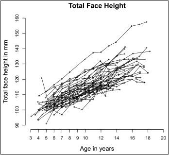
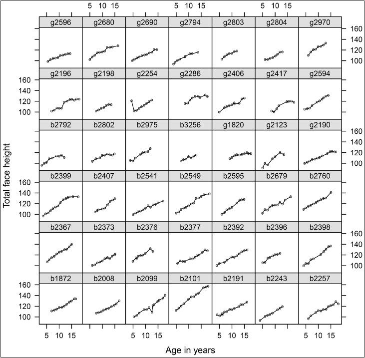
Figures 1 and 2 seemed to suggest that although growth in total facial height followed a linear pattern for some children (eg, girl 2596 and boy 2243 in Fig 2 ), growth in facial height accelerated at certain times for others (eg, boys 2407 and 2398); for some children, growth in total face height seemed to reach maturity around puberty (eg, girl 2196 and boy 2802). Simple regression calculates 1 intercept for all patients, whereas multilevel modeling allow for baseline total face height to vary (as expected naturally) from patient to patient. In our example, the intercept is the estimated total face height at birth for each participant. The multilevel modeling begins with the random intercepts model in which growth in total face height is assumed to be linear: ie, total face height at birth is allowed to vary (random intercepts) among participants, but all children have the same growth velocity for total face height after birth. The equations for the random intercepts model can be written as follows:
where TFH ij is the total facial height measured for subject j on the i th follow-up, Age ij is the chronologic age for subject j on the i th follow-up, b 0j is the intercept for subject j , b 1 is the regression coefficient for Age (which shows how total face height increases with age), e ij is the residual error term (which shows the differences between the observed total face height and the predicted total face height for subject j on the i th follow-up), β 0 is the average intercept at birth, and u j is the random effects for the intercept (the variation in estimated total face height at birth). The additional random intercept u j estimates unique total face height at birth for each subject, and it is assumed to follow a standard normal distribution.
Our results showed that the estimated average baseline total face height ( β 0 in equation 2 ) is 89.4 mm, and the average growth in total face height ( b 1 ) is 2.51 mm per year. The standard deviation for the random effects ( u in equation 2 ) is 5.75 mm, indicating that the estimated range of baseline total face height for these children was approximately between 78 and 100 mm. Figure 3 shows the fitted linear growth curves and the observed values for total face height, and some apparent discrepancies suggested that the random effect model (equation 1 ) was too simple for describing the total face height growth curve. This is not surprising because the assumption that all children have the same growth velocity for total face height is unlikely to be true. Next, we used a random slopes model to allow for different growth velocity (slope) for each child. The equations for the random slopes model can be written as follows:
Stay updated, free dental videos. Join our Telegram channel
VIDEdental - Online dental courses


