More Mechanical Testing
Mechanical testing is the basis of much of the research and development of dental materials (as elsewhere). More elaborate service loading conditions require extension of the basic ideas already presented. It is the purpose of this Chapter to explore such ramifications and present methods of comprehending the behaviour of these more complicated conditions for further insight.
Chapter 1 discussed the major basic topics of the behaviour of bodies when tested to determine mechanical properties. A number of aspects have been developed subsequently, in Chapters 4, 20 and 23 in particular, but there are further topics that are of direct interest to dental systems, or which help to clarify certain relationships and behaviours.
§1.Shear
Shear is often treated as if it were a completely separate mode of loading from tension and compression. Indeed, for simplicity we have spoken in just such terms in several places (Fig. 1§1.2, 1§2.5, 23§2.1), although the fact that it arises in what may at first seem simple conditions of compression (1§6.2, 1§6.3) or tension (Figs 11§5.4, 11§6.8) might be taken as indicating something more complex. The caption for Fig. 1§5.2 is another such indicator, that is, in a photoelastic model, where the situation in a body in compression is mapped entirely in terms of shear stress. It is therefore appropriate to consider such a system in a little more detail.
•1.1 Equivalent forms
Taking as a starting point the shear in a solid body of square cross-section between parallel planes as in Fig. 1§2.8, or even of a fluid body (Fig. 4§3.3), it is evident that as drawn there is a turning moment (Fig. 1.1 a), as can be understood from Fig. 23§1.2. Obviously, in a static test in which such a loading is attempted, there is no continuous rotation. Newton’s Third Law of Motion again decrees that there be an equal and opposite reaction, in this case an opposing moment couple. Whether or not this is arranged deliberately, it is clear that the loading device must provide the necessary constraint; the test machine is expected to be rigid enough to achieve this (the fact that for convenience we usually ignore such forces does not mean that they do not exist). We therefore have the situation depicted in Fig. 1.1 b.
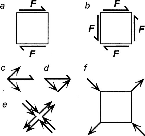
Each of the surface traction forces F, for example that on the top surface, may be resolved into two equal, orthogonal components (i.e., at right angles) (Fig. 1.1 c), symmetrically arranged with respect to F, the lower of the two being at -45° with respect to the horizontal direction. Thus, the magnitude of the component directed at + 45°, fx, is given by:
< ?xml:namespace prefix = "mml" ns = "http://www.w3.org/1998/Math/MathML" />
and the complementary fy by
(because for θ = 45°, and sin θ = cos θ = l/√2). We may check the magnitude of the resultant for this special case of orthogonal vectors using Pythagoras’ Theorem:
where the symbol ⊕ means vector addition (not just arithmetic addition). Such resolved vectors may be redrawn as if acting individually at each end of the original vector (Fig. 1.1 d) without loss of meaning. This pattern of vector resolution may be repeated at each face in turn, resulting in paired sets of diagonally-directed vectors (Fig. 1.1 e) equivalently applied at each comer of the original body (Fig. 1.1 f). The net comer-applied vectors then have magnitude 2 F/√2 = F√2, but with opposite signs from the point of view of the body: the one diagonal is subject to tension, the other to compression. Thus the pure, facially-applied shear of Fig. 1.1 b is found quite naturally to be equivalent to the application of identical tensile and compressive forces along the diagonals of the square, and vice versa.
•1.2 Mohr’s circle
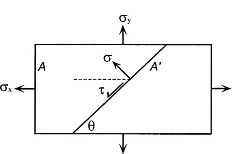
Another view may be taken by considering the equilibrium of a body in simple uniaxial tension (Fig. 1.2) in terms of the resolution in the x and y directions of the shear (F||) (i.e. parallel) and normal (F⊥(i.e. perpendicular) forces acting on a plane inclined at an angle θ to the load axis.
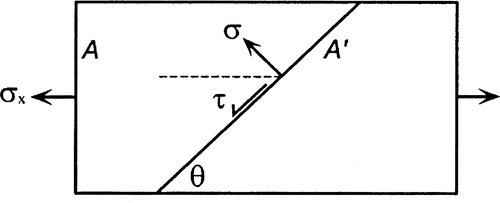
Given that Fy = 0, and A = A′.sin θ, dividing by the area of the plane, with a little rearrangement we have in terms of stresses
which by substitution and some trigonometric identities lead to
The stresses thus vary sinusoidally with θ (Fig. 1.3). Notice that since there is no distinction to be made between planes 180° apart, a natural symmetry, the right-hand half of such a plot is redundant. These two values (equations 1.6) can be plotted as a coordinate pair (σ, τ) as a function of θ, that is, in a parametric plot. This yields the plot shown in Fig. 1.4: a circle, tangent to the ordinate. This graphic expression of the relationship between the shear and normal stresses acting on a plane in a body is known as Mohr’s circle.
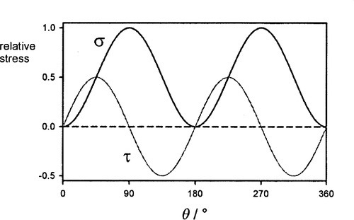
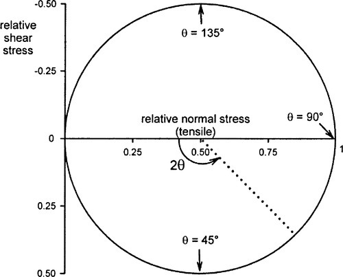
Some properties and implications can be identified immediately. Even with simple uniaxial tension, the body is subject to shear at all angles except parallel to the load axis, the maximum of which is precisely half the value of the maximum tensile stress, and this occurs at θ = 45°. The centre of the circle, whose radius R = σx/2, is therefore at (σx/2, 0), while at θ = 0° there is neither tension nor shear acting. More generally, the state of stress (σ, τ) for a point within the body, and at any plane orientation through it, is found to lie on that circle.
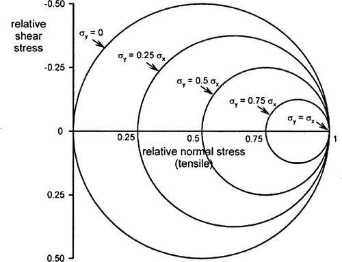
If, now, a second tensile stress is applied to the body, orthogonal to the first, to create a state of biaxial tension, the same kind of analysis can be applied, allowing for the additional stress components acting on the plane (Fig. 1.5).
which can be seen to reduce to equations 1.6 for σy = 0. The two terms for the normal stress are 180° out of phase, corresponding to the fact that the applied tensions are at right-angles. The effects of increasing the transverse tension are illustrated in Fig. 1.6: the maximum tensile stress is the greater of the two components, the minimum, the lesser of the two. It can be seen that the maximum shear stress depends on the difference between the two principal stresses. However, as the two tensions approach equality the maximum shear stress decreases, eventually to vanish at σy = σx; the circle diminishes to a point. This is the two-dimensional equivalent of hydrostatic loading, equibiaxial stress, when there is no change of shape, only of area (cf 1§2.6). We therefore notice that, quite simply, we have:
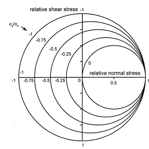
If instead of applying a tensile transverse stress it is made compressive instead, we use the same equations but treat the compression as a negative tension. This leads to the conditions illustrated in Fig. 1.7: the left-hand limit, the maximum transverse stress, moves leftward to correspond to the chosen value of σy as before, while the maximum relative shear stress naturally increases to ± 1 when the axial stresses are equal in magnitude and opposite in sign, as indicated by equations 1.8. This corresponds exactly to the conclusion of §1.1, the state of pure shear.
Stay updated, free dental videos. Join our Telegram channel
VIDEdental - Online dental courses


