Mechanical Testing
One of the central requirements of any product in service is that the mechanical properties are suitable to the task. We may view mechanical testing as an attempt to understand the response of a material (deformation, failure) to a challenge experienced in service (loading). A range of relevant mechanical properties are described, introducing the terminology and interrelationships, as well as some of the tests themselves that are used to measure those properties in the laboratory. Much advertising reports the comparative merits of products in terms of these test data, and unless the tests are properly comprehended – and their limitations recognized – sensible buying and application decisions cannot be made in the clinic or laboratory.
The challenges experienced by materials in dentistry extend beyond masticatory forces acting on restorations and prostheses. There are the deliberately applied forces such as in the deflection of a clasp as it moves over the tooth before seating, the seating of a crown, in rubber dam clamps and matrix bands, and in orthodontic appliances. In the laboratory, casting requires the hot metal to be forced into the mould, which must then be removed by mechanical means. In either context, shaping and finishing involves the application of forces through various tools, including the preparation of teeth and models.
The responses of the materials of greatest concern include the deformation, both reversibly and irreversibly, and the outright failure in service or in preparation. Thus, reversible or elastic deformation is important in controlling the shape and continued functioning of a device whilst under load. Equally, whatever deformation occurs here should only be temporary: permanent deformation would ruin dimensionally accurate work. Undesired permanent deformation is a type of failure, but cracking and collapse is plainly not intended in many cases. Yet cutting, shaping and finishing, the debonding of orthodontic brackets and other procedures involve intentional breakage. These too must be understood to be controlled.
In normal service, except for dropping or traumatic events, loads are not instantaneous, one-off events – they have a duration, and are usually repetitive. This means that the time scales of loading and of the response mechanism must be considered, as well as the pattern of loading in the sense of fatigue.
The fact that a wide range of types of property are of interest to dentistry means that product selection must be based on a consideration of all of them. The problem is that not all can be optimal in the intended application, and some may be undesirable. The essence of this is that compromise is always involved, trading a bad point for a good, or putting up with a less than perfect behaviour in one respect to avoid a disaster in another or to ensure better performance in yet another. This theme recurs in all dental materials contexts.
The purpose of mechanical testing in the context of dental materials, as with all materials in any context, is to observe the properties of the materials themselves in an attempt to understand and predict service behaviour and performance. This information is necessary to help to identify suitable materials, compositions and designs.[1] It is also the most direct way in which the success or failure of improvements in composition, fabrication techniques or finishing procedure may be evaluated. The alternative would be to go directly to clinical trials which, apart from being very expensive, time-consuming, and demanding of large numbers of patients (of uncertain return rates for monitoring) in order that statistically-useful data be obtained, would provide the ethical problems of using people in tests of materials and devices which could possibly be to their detriment. Laboratory screening tests used at the stages of development and quality control are thus cheaper, easier, faster and (usually) without ethical problems. The results of such tests are generally the only information on which to base decisions. The comparison of products and procedures, to aid in the choices to be made at the chairside, are also informed by such data in publications in the scientific literature. It is therefore a prerequisite to understanding mechanical properties in general, and the basis of recommendations for clinical products and procedures in particular (making rational choices of materials and techniques), that the tests which are employed to study them, as well as their interpretation and implications, be understood thoroughly.
§1 Initial Ideas
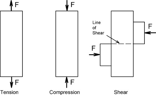
We are all too well aware that things break (Fig. 1.1). Such breakages can be costly, even dangerous to patient or operator, and certainly an inconvenience, at the very least. Evidently, in such examples the forces applied were in excess of the objects’ capacity to carry them. What needs to be understood, therefore, is what controls such behaviour: what is meant by strength, what determines it, how we can avoid exceeding it during use. Can we judge what is normal usage, what is abuse? Such damage does not arise spontaneously, but it depends on the forces acting during use. That is, the magnitudes, locations and directions of the loads applied, whether these were as intended by design, or inappropriate by accident or ignorance.

There are several types of loading that an object or body may experience in practice: for example, tension, compression and shear (Fig. 1.2). We can therefore envisage that there will similarly be a number of ways or modes of testing which might be used in an attempt to understand the response of bodies to such loads in service. But even if such loading is externally realistic, and thus said to be modelling service conditions, it will be found that the internal conditions may be considerably more complex. All three kinds of loading are typically present in any test, and they vary in intensity from place to place within the test piece. The interpretation of the results of such a test must therefore be done with care.
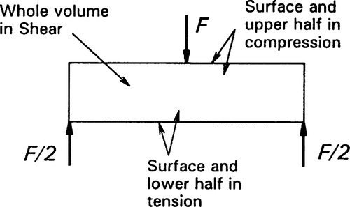
In a three-point bend test, for example (Fig. 1.3), we can identify a region where the principal result of the applied load is compression (extending from about the middle of the thickness of the beam to the concave surface), and a region in tension (similarly extending to the convex surface), but the entire region between the supports is in shear as well. This bend test thus gives us information about the performance of the material under those particular conditions of loading, but it may not say very much about any other circumstances. The deformation behaviour of the test piece certainly reflects contributions from all three aspects of the loading, although failure – meaning plastic deformation or crack initiation leading to collapse – may be attributable to one mode only. In the three-point bend beam case it is likely to be due to the tension on the lower, convex surface.
At the outset, then, we find that a major factor in testing materials is to match the conditions under which they will be put into service. Here, we are concerned about the mode of loading. This of course depends on an analysis being done of the service conditions themselves in order to determine what will occur and what will be relevant. It is this kind of thinking that underlies the selection of materials for particular purposes.
•1.1 Need to define properties
Now while we are perfectly capable (at least in principle) of determining the load that would cause a certain amount of deformation or even the collapse or failure in any sense of almost any given object, this in general is not a useful approach. There are an infinite number of possible shapes and sizes of object that might be put to some practical use, to say nothing of the variety of materials from which they could be made. The tabulation of such results would be impossibly cumbersome for even a small proportion of cases. Accordingly, a primary goal of materials science is to understand material behaviours in an abstract sense, that is, independent of shape and size. Thus, the underlying postulate of consistency1 is that
a given material under chosen conditions will always
behave in the same way, if subject to the same challenges
no matter what shape or size the object in which it is found. Notice that this is treating a material as having extent, as being a continuous but generalized ‘body’. This is to distinguish material properties from the even more abstract sense in which the chemical and physical properties of substances are understood – the behaviour of matter itself – without any sense that we need be handling objects.
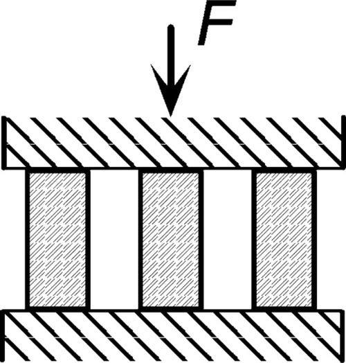
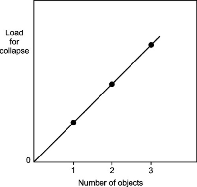
Consider an object that has an increasing compression load applied to it (as in Fig. 1.1, centre) until it collapses. We might term the ability of that object to carry a load without collapse the bearing capacity. Intuitively, this is what we need to know about any object that is meant to be load-bearing in any sense if we are to avoid overloading it. In other words, to determine if it is fit for duty under the conditions to which it will be exposed. Then, apply the same manner of loading to two, then three identical objects simultaneously (Fig. 1.3). Our elementary expectation is that the bearing capacity of the assemblage of objects will increase in a strictly linear fashion (Fig. 1.4). We naturally assume that each object carries its share of the load. We would therefore deduce that it is strictly unnecessary to test more than one such object at a time – there is no more information to be had in the multiple object test. Now, a little thought might suggest that perhaps in some sense it was the cross-sectional area of the set of objects being tested that was the underlying controlling variable. We should, for example, expect the same results whether we tested cylinders or rectangular objects – just so long as the cross-sections were the same.
Accordingly, our first efforts are directed to defining the mechanical properties of materials in just this size- and shape-free, abstract sense. We may therefore be in a better position to tabulate data in reference collections, having made the problem tractable. The intention is then that using such data we may calculate the expected behaviour of any arbitrary but real object, taking into account its shape and size, in order to determine its suitability or otherwise in a given application or circumstances. At the risk of being overly simplistic, materials science is about understanding such abstract properties as they affect the behaviour of objects, engineering is the design of real objects using that information. We shall return to consider the effects of shape in Chapter 23, indicating briefly how this is done.
Before proceeding, a distinction can be made with value. A mechanical property is limited to expressing the response of a material to externally applied forces in a scale-independent (that is, intensive) manner. In contrast, a physical property of a substance, compound or material, is an intensive character dependent on the spatial disposition of its matter (e.g. density), its response to a change in energy (e.g. thermal expansion coefficient), its effect on radiation (e.g. refractive index), or its effect on or response to fields (e.g. dielectric constant). This separation permits a clearer sense of the interactions occurring when we use or test materials.
§2 The Equations of Deformation
Perhaps the first inquiry to be made about the response of bodies to applied loads is the resulting deformation, the change in shape. In a great many aspects of dentistry it is the resistance to deformation – or the lack of it – that controls the suitability of a material for the application. Thus, the success of a partial or a full denture depends in part on its rigidity, but orthodontic devices must have readily-flexible components to do their intended job.
If a deformation is small enough then Hooke’s Law2 applies. This relates a deformation, for example the change in length of an object, L, to the force applied, F, through a spring constant, K (Fig. 2.1):
< ?xml:namespace prefix = "mml" ns = "http://www.w3.org/1998/Math/MathML" />

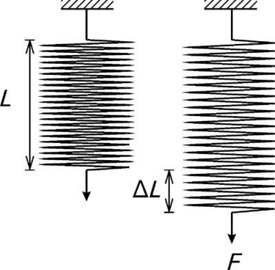
This force, for the moment, will be taken as acting in one axis only, i.e. the force is uniaxial. The spring constant here is relevant only to that particular test piece, and to no other, because it ‘hides’ the information about the length and cross-sectional area, even the shape, of the particular specimen.
•2.1 Stress and strain
To make things simple to start with, we first restrict the discussion to an object that is of uniform cross-section, that is, every section through the object perpendicular to the axis in which the load is applied is constant in both shape and area. We then imagine that the applied force is distributed uniformly over the entire cross-section at the end of the piece. We may now define stress, σ, as being force per unit area, A:

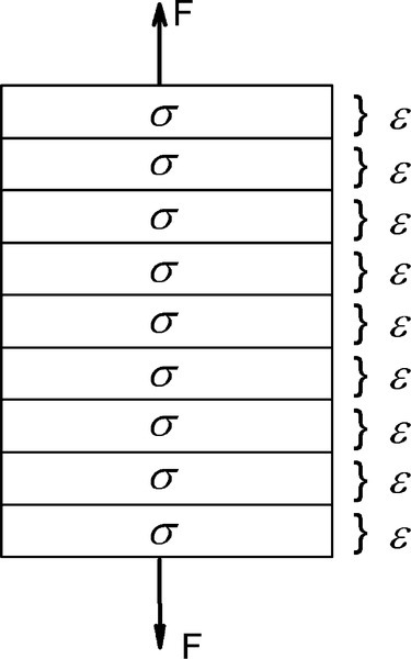
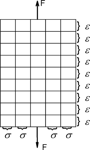
However, if the material from which the body is made is homogeneous, uniform in composition and structure throughout, we have a reasonable expectation that the response of every part to the forces acting will be similar. Thus, the stress acting on each layer of the piece is expected to be identical, transmitted from layer to layer unchanged and uniform (Fig. 2.2). This may be called the principle of uniformity, and is a version of the postulate of consistency.
To define the response of a unit portion of the body to the applied stress, we define strain, ε, as the change in length per unit original length, Lo:
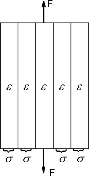
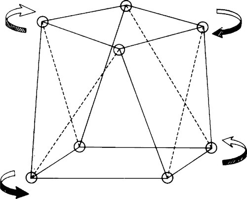
This is on the basis of the principle of uniformity again: each layer is expected to respond to the applied stress in identical fashion. Similarly, this principle may be applied to the body divided into separate columns (parallel to the load axis). Not only do we anticipate that every unit area column within the body will behave identically, we have no reason to expect that any portion of such a column will behave any differently from any other portion (Fig. 2.3). To see this, consider their behaviour if the columns were not joined to each other: there can be no change. This is because the situation is then as depicted by Fig. 1.3.
These two views (Figs 2.2, 2.3) can be combined to show that all regions of a body subject to uniform loading, must behave in identical fashion (Fig. 2.4). Therefore, identical stresses and identical strains occur at every point.
It can now be seen that in defining stress and strain both the applied load and the resulting deformation have been scaled by the dimensions of the object, to make its actual shape and size irrelevant. Hooke’s equation can therefore be reduced to a form which is, in principle, applicable to a test piece of any size and shape (but considering only regions of constant cross-sectional area and shape along the load axis). This version of Hooke’s Law says that the stress (substituted for force) is proportional to the strain (instead of change of length overall), with E as the new constant of proportionality:

Instead, therefore, of having to consider the behaviour of all kinds of shapes and sizes of bodies, we are now able to consider the behaviour of the material from which they are made, independently of size and shape. But, of course, from such data we can now calculate the response, if we so choose, for any other size and shape, not just that which was tested to get the data in the first place.
Care has to be taken to ensure that these defined terms are not confused as they are in ordinary, non-technical usage. The language of materials science, as in science in general, depends on the agreed definitions of such terms for effective communication.3 The units of stress are N/m2, or Pa, whereas strain is a dimensionless quantity, being the ratio of two lengths (in this example; there are also areal, volumetric and shear strains which could just as easily be considered in precisely the same manner).
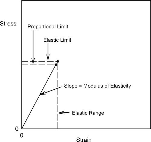
The graphical expression of Hooke’s Law is that the plot of stress against strain is a straight line (Fig. 2.5), the slope of which is the constant of proportionality between the two variables. The experimentally determined value of the slope of this line, E, is known as Young’s modulus or the modulus of elasticity, which from equation 2.4 a is therefore defined by the ratio of stress to strain:

This quantity is therefore a measure of stiffness or resistance to deformation of the material.
Sometimes it is more convenient to think in terms of the reciprocal property, the flexibility of the material (sometimes called “springiness”), in other words the deformation obtained for unit applied stress:
The term compliance, symbol J, is commonly used for this.
If the stress were to be increased still further, we might see the plot deviate from a straight line. We may then define another quantity from a stress-strain plot: the maximum stress which may be applied and still have the proportionality hold is known as the proportional limit. We have now to draw a very important distinction: that between the elastic limit and the proportional limit. The proportional limit is, as has been stated, the limit to which Hooke’s Law applies, up to which strict proportionality between stress and strain holds. It is implied that the behaviour is elastic; that is, the piece will return to its original dimensions (zero strain) when the stress is reduced to zero.
This essential condition – zero strain at zero stress after the temporary application of a stress – is a sufficient definition of elasticity. However, it says nothing about the kind of deformation behaviour shown by the piece under stress. There is no obligation for strict proportionality between stress and strain. In fact, in some classes of material (elastomers, for example, Chap. 7) proportionality cannot be observed (see also §13). Even so, many other materials, such as metals and ceramics, show a substantially linear region in a plot of stress against strain and therefore may be considered to approach ideal Hookean behaviour sufficiently well. But some metals, for example, show a more obvious deviation from ideality: a region of proportional deformation is followed by a small non-Hookean but still elastic deformation. We must therefore state that although under many circumstances the elastic limit is indistinguishable from the proportional limit, the elastic limit is always the higher of the two if there is a difference. Equally, the proportional limit may be zero, i.e. non-existent, for some classes of material. The important point is the fundamental distinction between the definitions.
In the field of orthodontics it is common to characterize wires in terms of the strain εmax observed at the elastic limit, σe, sometimes confusingly called the maximum flexibility or springback, and explicitly defined by:

A clearer term for this is elastic range. Thus, the strain at the elastic limit indicates how much deformation may be tolerated before the test piece will not return to zero strain when released. This needs to be known to avoid overloading a spring, for example. This quantity may also be found to be called the “range” (without further qualification). It can be seen that this assumes that the proportional limit and the elastic limit are the same, although for many metals the difference is not very great. These kinds of usage re-emphasize the need for very great care in reading and interpreting the dental literature, where technical definitions are often weak and terminology confused. This is not to say that the ideas themselves are not useful in certain contexts, but that the terms and their exact meanings may not be immediately obvious.
•2.2 Poisson Ratio
Experimentally it is commonly found that if a test piece is loaded in tension or compression, then, in directions perpendicular to the load axis, corresponding lateral strains will appear: a contraction if the load is tensile, an expansion if it is compressive (Fig. 2.6). This is known as Poisson strain. The behaviour under tension and compression is quite symmetrical, always so long as the deformations are small. The co-variation of lateral and axial dimensions is expressed through the Poisson ratio, v. This material constant, also known as a modulus, is the ratio of the lateral strain to the axial strain, but given a negative sign because the strains themselves have opposite signs:

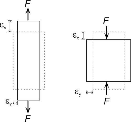
This is adopting the convention that the x-direction is the load axis, and the y-direction is perpendicular to that. Values of v for typical metals and ceramics lie in the range 0.2 – 0.4. On grounds of uniformity, as above, we expect the response will be similar in all directions perpendicular to the load axis, and in particular that:

where the z-direction is, as usual, mutually perpendicular to the other two.
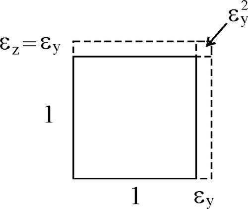
The definition of stress (equation 2.2) does not actually specify when the area is to be measured. We might assume, for example, that it is the original value, A, just prior to starting the test, that we should take. Yet it is plain from the mere existence of a non-zero Poisson Ratio that under stress the cross-sectional area of the test piece will change during the test, even if it remains within the (apparently) linear elastic range. We may explore the consequence of this changing area. The area A´ after deformation is given by:
where ΔA is the change in area. However, εy = ‐ ν. εx (from equation 2.5) and  may be ignored as it is very small (Fig. 2.7), so that we have:
as a good approximation. Therefore, at any point in the test, the actual stress,  , is to be calculated from the cross-sectional area A´ at that moment:
where σx is the stress calculated for the original cross-sectional area. Hence, the true modulus of elasticity, Eo, is given by:
It can be seen that Eo is very slightly larger than Young’s Modulus (E) since this latter is determined experimentally only using a measurement of the original area. The Poisson Ratio is typically about 0.3 for a metal and so is not a negligible parameter if a full description of a material’s behaviour is sought. Equation 2.10 also shows that the true stress-strain plot cannot in fact be exactly a straight line because of the extra term in the denominator. Nevertheless, it would in general be somewhat impractical to measure the lateral strain of specimens routinely (elaborate and delicate equipment is necessary), and it is usually sufficiently accurate – certainly easier – to employ the original area and just calculate Young’s Modulus, using what is known as the nominal stress, i.e. from Equation 2.2.
The remark “if the deformation is small enough” made for Fig. 2.1 needs a little amplification. In essence, it means that calculations are made on the assumption that the geometry remains unchanged in respect of anything that affects the calculated outcome. Generally, this may be effective as a working approximation, but clearly it has its limitations and these must be recognized – and checked – in all relevant contexts.
•2.3 Volumetric strain
From a knowledge of the magnitudes of the axial and lateral strains we can also calculate a volume strain, εv, that is, the relative change in the volume of the test piece. Thus, taking the new volume V′ to be the original volume V plus the change in volume, ΔV, its value can be calculated from the usual expression for the volume of a cuboid in terms of the lengths of its sides. Thus,
but
so that from equation 2.6:
Multiplied out, this has given a lengthy cubic expression, but because the strains themselves are typically very small in materials such as metals and ceramics, the quadratic and cubic terms can be considered negligible (see Fig. 2.7); that is, only the first three terms on the right need be considered. The error is only about the order of the square of the lateral strain. Subtracting the value one from each side we then have:
We thus obtain an expression for the volume strain in terms of the axial strain and Poisson Ratio. What this means is that for values of ν < 0.5, which is normally the case, there will be a change in volume of the piece when it is under load.
•2.4 True strain
Even the definition of εx itself needs refinement for it to be completely accurate, the point being that each increment of strain should be calculated in terms of the immediately prior value of the length of the specimen. In the limit, this requires the use of some calculus. So, considering the increment of strain at any moment, we can write

which is the limiting version of equation 2.3. When the specimen has been deformed elastically to the new length L, the true total strain ε* is obtained by integration:
then, since L = Lo + ΔL,
This means that the true strain is slightly smaller than the nominal strain for tension, and slightly more negative for compression, as a few trials with a calculator will easily show. If the deformation is small enough it can be seen that ε*  ε. In other words the approximation of equation 2.3 may be entirely adequate. However, to indicate that approximations are involved, σx and εx are sometimes referred to as engineering stress and engineering strain, to distinguish them from the true values. This also indicates that it is a matter of simple practicality in taking that approach. Most graphs of “stress” vs. “strain” are therefore in terms of these nominal stress and nominal strain values, unless they are explicitly labelled otherwise. We are prepared to compromise with the slightly less accurate values because of the expense and difficulty of obtaining the true values. However, one must not lose sight of the existence of Poisson strain.
•2.5 Shear
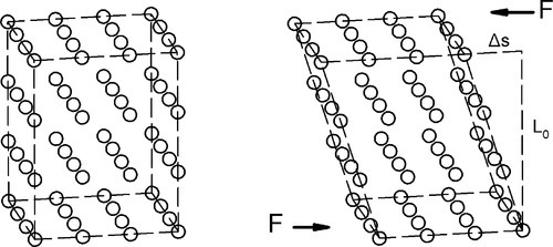
After the simple uniaxial tests discussed above, i.e. tension and compression, the next most important mode of testing is in shear (Fig. 2.8) where the layers of atoms or molecules of the material are envisaged as sliding over one another. The related mode of testing in torsion (Fig. 2.9) may be viewed as a particular case of shear. Shear is a common type of stress. For example, it is an aspect of the loading of beams in a three-point bend (Fig. 1.2). It is also relevant to the loading of interfaces such as between a bonded orthodontic bracket and a tooth, where the force is applied in the plane of the layer of cement. Endodontic files are ordinarily loaded in torsion in use, even though there is usually bending as well. There are many other examples.
In studying shear we are interested in the relative displacement of one layer sliding with respect to the next (Fig. 2.10). So, in a way analogous to that for direct uniaxial loading, we measure the length (Lo) over which the load is acting and the amount of displacement, Δs, at a given load, measured in the direction of load application. A version of Hooke’s Law applies here also, where the shear force is related to the displacement by a shear spring constant, Ks:

We can therefore define shear stress, τ, as the force per unit original cross-sectional area in the direction of shear:

and the shear strain, γ, as the displacement per unit original length over which the shear stress is applied, that is, the depth, the distance between the top and bottom layers:

Both of these are entirely analogous to the definitions for uniaxial loading. In particular, it can be seen that the shear stress on each layer is the same, and the relative displacement of each layer with respect to its neighbours must also be the same.
The shear modulus of elasticity, G, is then defined simply by:

The reciprocal of this is known as the shear compliance, which is analogous to ‘flexibility’ (equation 2.4 c). It can also be shown that this shear modulus is related to Young’s Modulus through the Poisson Ratio:
It is therefore not necessary to measure both moduli experimentally. To understand shear deformation we can use Young’s modulus. Alternatively, it may be difficult to measure Young’s modulus, yet the shear modulus might be easy to determine. However, either way it requires a knowledge of the Poisson ratio.
Two other points emerge from this. Firstly, the shear stress is the same on every layer, all the way through the specimen. The force acting over any layer is transmitted undiminished to the layer below. Secondly, on the principle of uniformity, the relative displacement of one layer with respect to the next must be the same for all layers in a homogeneous specimen.
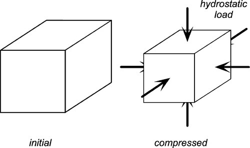
•2.6 Bulk modulus
Using similar reasoning, the behaviour of materials under hydrostatic loading can be described with the bulk modulus, B (again, it is understood that this is a type of elasticity). Under hydrostatic loading – in which the pressure (i.e. stress) on the sample is uniform in all directions – there is no change of shape, only of volume (Fig. 2.11). Again, the bulk modulus is related to the more easily measurable Young’s Modulus:
The reciprocal of this quantity is also known as the compressibility, κ, of a material:
If we combine equations 2.22 and 2.23 we get the following:
which illustrates the interdependence of the three moduli of elasticity.
•2.7 Effect of structure
We have so far assumed that the materials being tested are uniform, homogeneous and isotropic. While this may be true enough for an amorphous material (such as glass, which shows no long-range order at the molecular level), many materials are crystalline (thus showing long-range order) or heterogeneous. The latter class of materials, known generally as composite materials, are dealt with in later chapters as they have their own special characteristics. A crystalline structure necessarily has directionality, there can be no such thing as spherical symmetry in this case and the properties of the material must be anisotropic. That is to say, the mechanical properties vary according to the direction chosen for the load axis since the nature (i.e. the stiffness and strength) of the atomic or ionic bonds themselves vary with direction. Hydrostatic loading of single crystals will often involve some change of shape, since the three mutually perpendicular strain directions are unlikely to be equivalent if they are chemically or otherwise distinguishable. In fact, some 21 separate elastic moduli can be defined to express all of the possible directional variability in properties. However, most crystal types do have certain degrees of symmetry and so in practice there are rather fewer independent moduli, that is, the minimum number of moduli which are not algebraically derived from each other.
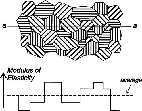
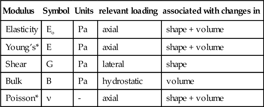
Even so, in dentistry we are very rarely, if ever, concerned with the properties of isolated single crystals. The materials we shall deal with are all polycrystalline (Fig. 2.12), such as metals, with usually random orientation of the individual crystals, or amorphous, such as glasses, when the local (at the atomic scale) anisotropies cancel out so that the overall effect is of an isotropic material. Because of these effects we can reduce the minimum number of moduli necessary to describe fully the behaviour of the material to just two: Young’s Modulus and the Poisson Ratio, because the others can be calculated from these two values (see Table 2.1). However, it must be emphasized that the validity of these properties in describing behaviour depends on the total deformations being small. Extremes lead to departures which require more complicated treatment.
§3 Plastic Deformation
So far we have dealt with the behaviour of materials for small deformations. This was to ensure that the geometry of the system was essentially unchanged, but also to keep the stress lower than the elastic limit. By definition, if a return to zero strain on removing the load is not obtained, there will have been permanent deformation, and thus the elastic limit will have been passed.
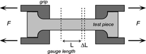
We may consider as a general example a specimen being tested in tension (Fig. 3.1), as this mode is somewhat easier to understand than compression (a tensile specimen will be assumed unless otherwise specified). The essential features of the test are that the specimen is gripped to apply the load, F, while a representative portion known as the gauge length, L (that is, the length of a representative portion before any load is applied), is monitored with some instrument (typically a strain gauge extensometer) to determine the change in length, ΔL for the load that is then applied. From the measurements of the initial cross-section dimensions and gauge length, the stress and strain can be calculated. The behaviour of a such a specimen can now be examined in more detail.
Thus, after stressing past the elastic limit, the material may enter its plastic range (Fig. 3.2). The deformation has gone so far that some atoms or molecules cannot return to their original posi/>
Stay updated, free dental videos. Join our Telegram channel
VIDEdental - Online dental courses


