Let’s assume that, for our study, we take a sample from the population of interest and we want to draw conclusions about the population based on the data from this sample. We only have one sample and therefore we do not know the true mean of the sampling distribution. In Figure 1 (sampling distribution from the population of interest), the blue stars on the red horizontal lines represent mean values of a single studies such as ours. We can construct an interval called the confidence interval (CI) around our single-sample estimate. This interval is given by our sample mean ± 1.96 standard error (SE).
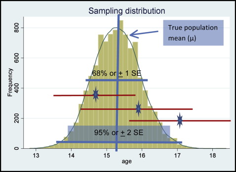
For example, the 3 red horizontal lines indicate the means and their 95% CI of 3 samples from the population of interest. The 2 top lines contain the true population mean (derived from the sampling distribution), whereas the bottom line does not contain the true population mean.
The only time this interval would not contain the true mean is when you are unlucky enough that the sample is at the tail end of the distribution. This should only happen 5% of the time when we use the 95% CI and is shown by the bottom red horizontal line in Figure 1 .
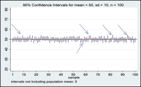
Attention should be paid to the interpretation of the 95% CI. It is commonly, yet wrongly, interpreted as a range that contains the population mean with 95% probability. The correct definition of the 95% CI is the following: if samples of the same size are repeatedly extracted from a population and their 95% CIs are calculated, then 95% of these CIs will capture the true population mean. Figure 2 shows the 95% CI concept, indicating that out of 100 samples (each, n = 100) drawn from a population with known μ = 50 and σ = 10 (for the variable of interest), only 5% of the samples are expected not to contain the true population mean in the 95% CI. Samples not containing the true population are indicated by the arrows in Figure 2 .
We have just illustrated the idea that, in theory, we could sample the population many times and obtain many different estimates.
However, in practice, we take only one sample from the population of interest. The idea of a sampling distribution is fundamental to statistical inference because it allows us to relate the one and only sample that we have actually collected to the true population value.
Now, let me summarize the steps to make statistical inferences from the sampling distributions using a numeric example. In Figure 3 , we have the sampling distribution of a large number of samples drawn from the population of interest (let’s say, adolescent orthodontic patients). The measurement of interest is age, and we can see that the mean of the sampling distribution is approximately 15.3 years, and let us say that this is the true population mean.
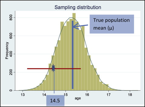
We calculate our sample mean, and it is 14.5 years (SD, 5.79 years), n = 74.
- 1.
The estimate (mean, 14.5 years) in our sample is only one of many estimates that could have been obtained from other random samples of the same size and that are represented by the sampling distribution above.
- 2.
The mean of the sampling distribution is the true population value μ (here, μ = 15.3).
- 3.
The standard error of the sampling distribution of a mean is σ√n
σ n
. For 1 sample of 74 patients, the standard error is SD√n=5.79√74=0.67
SD n = 5.79 74 = 0.67
, where the standard deviation was calculated from our single-sample data. - 4.
The sampling distribution is normal when the sample size is large. We know that about 68% of a normal distribution lies within about 1 SD, and that 95% lies within 2 SD (more precisely, 1.96 SD) of its mean. The standard deviation of a sampling distribution is the standard error. So we know that 95% of means estimated from samples of 74 will lie within 15.30 + 1.96 × SE = 15.3 + 1.96 × 0.67, or 13.99 and 16.61). As the sample size increases, the standard error and the calculated range become smaller, and we say that we have more precision.
Finally, we only have one sample from our study; therefore, we do not know the true mean of the sampling distribution. Our sample mean is 14.5 years, and we can use it to construct an interval (called a confidence interval) around our sample mean ( Fig 4 ).