Introduction
The purpose of this study was to analyze the relationship between the mandibular dental and basal bone arch forms for severe skeletal Class III patients by using 3-dimensional digital models.
Methods
Thirty-three virtual pretreatment mandibular models were created with a laser scanning system. The most prominent part of the center of the clinical crown where an orthodontic bracket would be placed (FA) and the most prominent point on the soft-tissue ridge at the mucogingival junction (WALA) were used to represent the dental and basal arch forms, respectively.
Results
A moderate-to-high correlation between the FA and WALA curves was found, especially in the canine ( r = 0.61) and molar ( r = 0.91) areas. The WALA curve’s radius of curvature in the anterior teeth areas was greater than that of the FA curve (WALA, 22.47; FA, 18.18). In the canine and molar areas, the coefficients of variation of FA (6.70%, 6.01%, 15.30%, and 9.97%) were greater than those of WALA (5.42%, 3.88%, 8.53%, and 7.22%). For the FA and WALA points, the coefficients of variation of the canine area were greater than those of the molar area.
Conclusions
Both curves were individualized. A moderate-to-high correlation was found between the dental and basal bone arch forms. Compared with the WALA points, the FA points are located more lingually. The individual differences were found to be significantly greater in the canine region.
Highlights
- •
Both dental and basal arch forms were individualized.
- •
A moderate to high correlation was found between the dental and basal arch forms.
- •
The basal bone arch can to some extent be used as a clinical guide for individualized archwires.
- •
Differences between dental and basal arch forms were greater in canine than in molar areas.
Dental arch form is an important element in orthodontic treatment and retention. During orthodontic treatment, excessive tooth movement over the basal bone may lead to periodontal complications and an unstable treatment effect. Most orthodontists have realized that expansion of the dental arch is affected by the shape of the basal bone arch.
In 1925, Lundström put forth the “apical base theory” to explain the boundaries of the expanding dental arch. He proposed that the supporting bones are not changed by orthodontic tooth movement or masticatory forces, and that their expansion is limited by the apical base bone. Tweed and Begg also found strong evidence for the limitation of dental arch expansion. In 1954, Howes demonstrated that the basal bone is the narrowest region of the alveolar bone, 8 mm below the marginal gingiva.
The relationships between the dental and basal bone arches and the different types of malocclusion models have been explored in several studies. However, little attention has been paid to severe skeletal Class III subjects. In addition, most studies have focused on analysis of the transversal dimension: eg, the measurements of intercanine and intermolar widths. In 2004, Tancan found that mandibular intercanine and intermolar alveolar widths were significantly greater in Class III patients using plaster models. This result also agreed with that of Braun et al.
Furthermore, Slaj explored the different malocclusions in 3 dimensions and found greater intercanine and intermolar widths in Class III subjects in the transverse dimension.
In addition, for severe skeletal Class III patients, orthognathic surgery is the best choice for correcting the skeletal deformities. However, skeletal relapse is the most common complication after orthognathic surgery, and some vital factors, such as dentoalveolar and soft-tissue changes, can lead to failure of the treatment. Another crucial element—dental arch matching—is equally important to the results. Another reason for the study was to explore the relationship between dental and basal bone arch forms in our orthodontic clinical practice.
Andrews and Andrews identified the WALA points as the most prominent point on the soft-tissue ridge at the mucogingival junction. The FA point was defined as the most prominent part of the center of the clinical crown where an orthodontic bracket would be placed in an appliance system. In several studies, the WALA and FA points have been used to refer to the basal bone arch form and the dental arch form, respectively. Although the association between dental and basal bone arches have been studied by using the landmarks of FA and WALA in Class I and Class II groups, their relationship in severe skeletal Class III patients remains unknown.
The purposes of this study were to explore the respective metric properties of mandibular dental arch forms and the supporting bone in subjects with severe skeletal Class III malocclusion and to establish the relationship between the natural dental and basal bone arch curves derived from the FA and WALA points.
Material and methods
The sample consisted of 33 pretreatment mandibular casts obtained from subjects with skeletal Class III malocclusion (21 female, 12 male; all patients were Mongolian). Their ages ranged from 17.07 to 23.47 years (17.07-23.23 years for females, 19.03-23.47 years for males; mean age, 20.27 years).
The inclusion criterions for the subjects were (1) severe skeletal Class III (ANB angle, <−5°), (2) minor arch-length discrepancy (crowding, ≤2 mm; spacing, ≤2 mm), (3) Class III canine and molar relationships, (4) all pretreatment models in good condition with no distortion or surface defects, and (5) plans included combined orthognathic and orthodontic treatments.
The exclusion criteria were (1) dental crowding or spacing >2 mm, (2) missing or decayed teeth or prosthetic crown, and (3) gingival defects or unidentifiable mucogingival junction on the model.
For the measurement and statistical analysis, a laser scanning system (R700 laser scanner; 3Shape, Copenhagen, Denmark) was used to scan the pretreatment mandibular casts at a resolution of 0.02 mm. The 3-dimensional (3D) data were imported from reverse modeling software (Rapidform 2006; INUS Technology, Seoul, Korea).
To evaluate the reliability of the FA and WALA point identifications, 10 models were randomly selected from the 33 samples. Interoperator reliability was examined between 2 operators (W.Z., J.W.). Intraoperator reliability was examined by selecting the FA and WALA points twice at an interval of 2 weeks and comparing the agreement. The intraclass correlations test (ICC >0.9) exhibited high reliability by both operators. The definitive values were defined as the average values from the 2 examiners.
The locations of the FA and WALA points were obtained. The reference points for each mandibular tooth from the right first molar to the left first molar on each 3D model were digitized to represent the dental and basal arches, respectively ( Supplementary Fig 1 ).
The FA point was defined as the most prominent part of the clinical crown center. For the first molar, the FA point was identified as the most prominent point near the line with the mesiobuccal groove.
The WALA point was determined by the most prominent point on the soft-tissue ridge immediately superior to the mucogingival junction.
To build the reference plane, the 12 FA points and the 12 WALA points from the right first molar to the left first molar were used, resulting in the location of all FA and WALA points in 1 plane. This reference plane is flat, meaning that we can transfer the FA and WALA points to the corresponding projection points in same height and create a smooth dental curve.
To establish the 3D coordinates, the 2 FA points of the 2 mandibular incisors were connected to create 1 line segment on which the midpoint was defined as FA1. WALA1 was created in a similar way. The points FA1 and WALA1 were connected, and the midpoint was determined to be the FW1 point. Then, FW1 was projected onto the reference plane, creating a projection point (FW1_ ref ). The point FW1_ ref is the origin with the coordinates (0, 0, 0). FA6, WALA6, FW6, and FW6_ ref were created in the same way ( Supplementary Fig 2 ). Three points (FW1_ ref , FW6_ ref , and FW6) were chosen to build the 3D coordinates (these can ensure the directions of these mutually perpendicular axes XX, YY, and ZZ).
To measure the distances between the FA_ ref points and the WALA_ ref points, all FA and WALA points were projected onto the reference plane ( Supplementary Fig 3 ), creating a number of projection points (FA_ ref and WALA_ ref ). The distances between FA_ ref and WALA_ ref for each tooth were exported into SigmaPlot (version 10.0), a statistical graphic software.
The widths between the FA and WALA points of the bilateral mandibular molar and canine areas were determined. The respective distances as projected onto the reference plane between the FA_ ref and WALA_ ref points for the bilateral canines and molars were measured and recorded as distance FA3, distance WALA3, distance FA6, and distance WALA6. The Pearson correlation was used to examine the associations of widths and ratios.
The curve fittings of the FA_ ref points and WALA_ ref points for the mandibular arch were determined. The scatter diagrams (created by subsequent projection points on the reference plane) of the samples were processed by nonlinear regression analysis with SPSS software (version 17.0; SPSS, Chicago, Ill). To compare and superimpose the arch forms, we can translate the curves along the y-axes without changing their shapes. Therefore, the data should be taken with the correction of the y-axis: to reduce the influence resulting from each coordinate and make the graphics more simple and intuitional, each point was shifted to the origin by deducting the value of the function’s y-intercept. After moving the curves along the y-axis, we could move these curves as close to the origin as possible. Through this method, the various curves with different origins can be presented in a much more organized way.
Because the distributions of the FA and WALA scatter plots were presented in rough symmetry, we chose an even-order power function for curve fitting. Comparing the correlation coefficient ( R 2 ) and the degree of fitting of scatters from the second, fourth, and sixth degrees even-order power functions, we chose the fourth degree even-order power function (y = a + x 2 /2r + b × x 4 ) as the best fitting curve representing the regular scatter points. The estimate of parameter ( a , r , b ), the coefficient of regression ( R² ), and the radius of curvature (at x = 0, the value of r ) were derived. The radius of curvature ( r ) can reflect the tooth location like an arc line in the anterior region: ie, the greater the value of R , the flatter the curve in the anterior tooth region; this makes it more similar to the square arch form. Otherwise, the fitting curve is more similar to a tapered one. The radius curvatures for the anterior tooth areas were recalculated for each model and analyzed with the paired t test.
The coefficients of variation (CV) of FA and WALA in the canine and molar areas were determined by evaluating the individual differences of tooth locations in the canine and molar areas. The linear interpolation method was used to calculate the CV of the mandibular canines and molars, and the CV values of the various areas and different vertical positions (FA and corresponding WALA points) were compared by statistical analysis.
Results
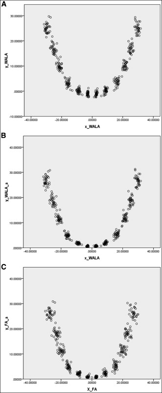
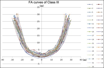
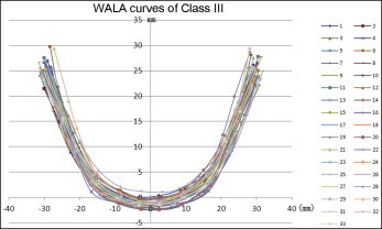
The projection points of the corresponding FA and WALA points were used to draw the curves for 1 subject ( Fig 1 ) and the superimposed curves for the Class III sample ( Figs 2 and 3 ).
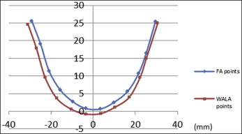
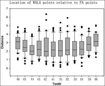
To determine the average relative distances between corresponding FA and WALA projection points, the distance between FA_ ref and WALA_ ref for each tooth from the right first molar to the left first molar was recorded and defined as the criterion of positive or negative value (if FA point was located more lingually, the value was positive; otherwise, it was negative). The data are displayed in Table I and Figure 4 .
| Tooth | ||||||||||||
|---|---|---|---|---|---|---|---|---|---|---|---|---|
| 46 | 45 | 44 | 43 | 42 | 41 | 31 | 32 | 33 | 34 | 35 | 36 | |
| Average | 3.00 | 2.55 | 2.16 | 2.42 | 2.51 | 2.24 | 2.32 | 2.49 | 2.34 | 2.34 | 2.83 | 3.20 |
| SD | 0.91 | 1.01 | 0.91 | 1.16 | 1.47 | 1.20 | 1.30 | 1.34 | 1.16 | 1.09 | 1.00 | 0.92 |
For the correlation analysis of the intercanine and intermolar widths for the FA and WALA points, the descriptive statistics for FA_ ref and WALA_ ref points for the canine and molar widths are shown in Table II . The values of 3 comparison groups (distance FA3 and distance WALA3, distance FA6 and distance WALA6, and the corresponding FA ratios and WALA ratios) were statistically analyzed with the Pearson correlation coefficient ( Table III ).
| FA6 | FA3 | WALA6 | WALA3 | FA ratio (3-3/6-6) | WALA ratio (3-3/6-6) | |
|---|---|---|---|---|---|---|
| Average | 54.05 | 30.49 | 59.30 | 32.03 | 0.57 | 0.54 |
| SD | 3.07 | 1.54 | 2.04 | 1.85 | 0.04 | 0.03 |
| FA6-WALA6 | FA3-WALA3 | FA-WALA ratio (3-3/6-6) | |
|---|---|---|---|
| Correlation coefficient | 0.910 | 0.614 | 0.637 |
| t value (degree of freedom n − 2 = 31) | 12.241 | 4.332 | 4.600 |
| P | <0.001 | <0.001 | <0.001 |
The curve fittings of the WALA projection points were determined. According to the original WALA scatter plot ( Fig 5 , A ), we can reduce the influence resulting from the individual coordinates by correcting the y-axis. Each coordinate on the y-axis should be deducted from a value of the y-intercept to approach the origin ( Fig 5 , B ). With these shifted new scatter points, we processed the data by nonlinear regression analysis with the fitting curves (y = 0.022x 2 + 8.80 × 10 −6 x 4 ). After correcting the projections, the final curve fitting resulted in R 2 = 0.963, indicating an extremely high degree of fitting ( Fig 6 , A ).