In the last article, we demonstrated how to use multilevel linear or curvilinear models to analyze longitudinal orthodontic growth data. Because facial growth tends to accelerate during adolescence, fitting a straight line is likely to miss some important characteristics in the growth data. Curvilinear models with higher polynomial terms, such as quadratic, cubic, or quartic for ages, are commonly used for fitting a nonlinear growth curve. The advantage of this approach is that with enough data points it is straightforward to fit a polynomial growth curve; however, when the degrees of polynomial terms increase, their regression coefficients become less straightforward to interpret. Moreover, even if the polynomial curve provides a good fit to the data, the regression coefficients might not provide information for some key events of clinical interest in the growth process. In this article, we use a simple example to show how an alternative approach to the curvilinear model—ie, the nonlinear growth model—might be useful for orthodontic growth data analysis. Nonlinear growth curve models have a long history in human growth research and have been implemented by many commercial and free statistical software packages. In this article, all our analyses were undertaken using the library nlme for the free statistical software R (version 2.15.3; R Core Team, 2013, Vienna, Austria).
We obtained data for 4 boys for whom serial cephalometric tracings were made between ages 6 and 7 years and up to age 19 years from the University of the Pacific Mathews Growth Study at the American Association of Orthodontists Foundation Craniofacial Growth Legacy Collection. Each child had 10 or 11 cephalometric tracings. The outcome of our nonlinear modeling was the growth in total face height.
Statistical analysis
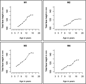
We first plotted the observed total face height for the 4 boys to examine the growth patterns. Figure 1 shows the 4 growth curves for total face height separately, and it became clear that the cephalometric tracings for total face height contained measurement errors; for some subjects, the total face height measured at later ages was smaller than that in early ages. Two other features also drew our attention. First, the acceleration in growth velocity for total face height seemed to start at adolescence, but the ages when this acceleration started and the magnitude in acceleration varied among the children. Second, growth in total face height seemed to reach maturity around late puberty, with substantial differences in the final adult total face height. Ideally, we would therefore like our nonlinear growth models not only to characterize those growth features but also to provide estimates for key attributes of the growth process: eg, the average growth velocity, the age with the greatest growth velocity, and the final adult total face height.
Logistic curve models
Our analysis began with a 4-parameter logistic curve model that relates total face height to chronologic age via a symmetric sigmoidal or “S-shaped” function. The equation for logistic curve model can be written as the following
T F H = h 0 + h 1 − h 0 1 + exp [ ( k − A g e ) / δ ]
Stay updated, free dental videos. Join our Telegram channel
VIDEdental - Online dental courses


