2
Functional and Technical Characteristics of Different Cone Beam Computed Tomography Units
Introduction
By providing three-dimensionally (3D) accurate representation of craniofacial structures, cone beam computed tomography (CBCT) has opened up new paradigms in diagnosis, treatment planning, and assessment of treatment outcomes in orthodontics and orthognathic surgery. This technology also has found applications in many other fields of dentistry, particularly in implant dentistry, imaging of craniofacial trauma, and facial reconstruction; additional applications are being envisaged in endodontics and periodontics. Useful medical applications of CBCT technology include imaging for otorhinolaryngology (ear, nose and throat [ENT]), skull base, radiotherapy planning, intra-operative imaging, angiography, and even mammography (Broderick et al., 2007; Miracle & Mukherji, 2009a,b; Angelopoulos et al., 2012).
CBCT, an X-ray–based imaging modality, is similar to multi-slice computed tomography (MSCT), also referred to as multi-detector computed tomography (MDCT), but with far less radiation exposure, reduced cost, and high spatial resolution (Miracle & Mukherji, 2009a). The increasing popularity of CBCT has been facilitated mainly by reductions in radiation and costs resulting from advances in flat panel detector (FPD) technology and processing power of computer hardware supported with advanced software applications.
Most CBCT scanners are intended for use in the imaging of the head and neck region. In 1998, the first CBCT machine for imaging of the maxillofacial region (Mozzo et al., 1998) was marketed for commercial use (Miracle & Mukherji, 2009a). By 2005, there were five manufacturers supplying CBCT machines. Currently, there are over 20 manufacturers providing over 40 different CBCT units (Molen, 2011; also see Chapter 6). These units vary in their configuration, hardware, and image reconstruction capabilities, which continue to evolve rapidly. The overall goal of this chapter is to provide the reader with a working knowledge of the capabilities and specifications of the broad array of CBCT scanners that currently are available. More specifically, this chapter compares and contrasts several of the commonly used CBCT units and discusses their relative merits for use in orthodontics. The review of CBCT scanners is preceded by some of the essential information on CT imaging, including a discussion of concepts such as resolution, noise, artifacts, and determinants of radiation exposure.
Characteristics of a CT Image
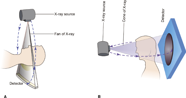
The principle of CBCT is the same as that of conventional CT except for differences in the type of beam used, configuration of the detectors, and reconstruction algorithms used (Figure 2.1). The use of two-dimensional (2D) FPDs in CBCT enables the scanner to obtain the required information of the region of interest (ROI) in a single rotation or, in some cases, in two rotations, which decreases the exposure time drastically relative to MSCTs. Depending on the equipment and reconstruction algorithm used, the scan arc can be 360° or less. In essence, the machine acquires multiple images of the structure at various angles during a rotation. The total number of images acquired depends on frame rate, speed of rotation, and scan arc. The greater the number of images acquired, the greater the radiation dose and the better the image quality. In contrast to MSCT, X-rays in CBCT are used more efficiently, which decreases the load on the X-ray tubes.
An image from a MSCT or CBCT has three fundamental characteristics or components that are common to all medical imaging techniques: (1) resolution, (2) image noise, and (3) artifacts. These, in turn, are controlled by machine parameters such as peak tube voltage (kVp), milliamperage seconds (mAs), scanning time, field of view (FOV), frame rate, speed of rotation, arc of the trajectory, type of detector, reconstruction algorithm, and radiation scatter. The effects of some of these machine parameters on resolution, image noise, and artifacts are summarized below and in Table 2.1.
Table 2.1 Scan parameters influencing image quality.
| Tube voltage (kVp) | High | Increased energy of the X-ray beam, increased tissue penetration, good signal to noise ratio |
| Low | Better contrast resolution, lower signal to noise ratio and lower dose for a given tube current | |
| Tube current (mA) | High | Good signal to noise ratio, thereby increasing the contrast resolution |
| Low | Lower patient dose, poor signal to noise ratio | |
| Scan time | Long | Prone to motion related artifacts |
| Short | Superior temporal resolution, fewer artifacts | |
| Field of view (FOV) | Large | Larger area is covered, lower spatial resolution |
| Small | Better spatial resolution | |
| Slice thickness | Large | Good signal to noise ratio, lower z-axis resolution |
| Small | Partial volume effect is reduced, poor signal to noise ratio | |
| Reconstruction algorithm | Smooth | Image appears smother and less noisy, spatial resolution suffers |
| High frequency | Better spatial resolution but noisier image |
Resolution
In medical imaging, resolution typifies the ability of an imaging modality to resolve closely placed objects. Resolution can be classified further into spatial resolution, contrast resolution, and temporal resolution (Mahesh, 2009).
Spatial Resolution
Spatial resolution is the ability of a scanner to distinguish closely placed objects. The better the resolution, the better the image quality. Spatial resolution is measured in two planes: axial plane (x–y plane) and longitudinal plane (z-axis). The key factors controlling spatial resolution in a CT scan are related mainly to receptor characteristics, focal spot size, detector size, scanner geometry, type of reconstruction filter used, and patient motion.
A major advantage of CBCT is the excellent spatial resolution obtained by the use of FPDs (0.4 mm or lower), which can provide isotropic voxels of high resolution up to 80 µm (0.08 mm) compared with 500–1000 µm voxels in MSCT. The current generation of CBCT scanners have the ability to acquire data at voxel size 0.08–0.4 mm (Angelopoulos et al., 2012). However, a machine with a smaller voxel size does not translate necessarily into higher clinical resolution. As the voxel size reduces, fewer photons reach each voxel, thus reducing the data acquired by each voxel. Due to tissue- and beam-related differences, adjacent voxels are affected by a different number of photons, resulting in an inhomogeneous image, which leads to loss of contrast and increased image noise.
The resolution power of a scanner is measured clinically by its ability to distinguish closely spaced bars in a CT phantom and is specified as line pairs per centimeter (lp/cm) or per millimeter (lp/mm; Mahesh, 2009; see also Chapter 8). Current CBCT scanners offer a resolution of as low as 5 lp/mm compared with 2–3 lp/mm for CT scanners (Angelopoulos et al., 2012).
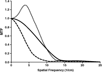
Modulation transfer function (MTF) is a more objective and quantitative way of determining spatial resolution. It is defined as the ratio of output modulation to input modulation and relates the percentage of actual contrast conferred to a spatial frequency of inserts in a phantom. MTF values range between 0 and 1 and usually are depicted graphically (Figure 2.2). Manufacturers often use 50, 10, 20, and 0% MTF to indicate the frequencies (lp/cm) corresponding to the points on the MTF curves (Mahesh, 2009). High MTF values in the low frequency range are needed to outline coarse details, while high MTF values in the high frequency range are necessary to portray fine details and sharp edges (Suomalainen et al., 2009). The data reported by most manufacturers on the MTF values are derived under experimental conditions using phantom heads. However, due to the many variables including the presence of soft tissues, artifacts, and patient motion, the resolving power of scanners under clinical conditions may be lower than that reported by manufacturers.
Temporal Resolution
Temporal resolution is the ability of an imaging system to discriminate several sequentially acquired projection data in time (Miracle & Mukherji, 2009a). A system with higher temporal resolution would have more contrast resolution. Solid state FPDs of CBCT systems have limited temporal resolution ability compared with ceramic detectors of MSCT systems (Orth et al., 2008), which limits the frame rate and contributes to streak artifacts, thus reducing low contrast detectability (Akpek et al., 2005).
Contrast Resolution
Contrast resolution, or low contrast detectability (LCD), is the ability of an imaging device to distinguish differences in tissue attenuation or the capability of an imaging system to distinguish objects from the background (Goldman, 2007; Mahesh, 2009). A system with high LCD has an increased capability to resolve objects from the background and, therefore, is considered to have high sensitivity. Contrast resolution is an important determinant of image quality. When the contrast resolution decreases, the visualization of tissue differences in the low contrast areas such as soft tissues becomes poor. CT contrast is measured on a scale of −1000 to 1000 Hounsfield units (HU). The major factors influencing contrast resolution include tube current, slice thickness, thickness of the region being imaged, detector sensitivity, reconstruction algorithm, and image display (Mahesh, 2009).
CBCT inherently has poor LCD, which results in suboptimal soft tissue imaging. CBCT systems typically have an LCD of 10 HU (Dörfler et al., 2008) compared with 1 HU resolution of modern MSCT (Miracle & Mukherji, 2009a,b). Despite this caveat, the visualization of high contrast structures such as bones is not affected in CBCT imaging. The prime cause of lower contrast resolution in CBCT is the scatter radiation, which is inherent to the geometry of the CBCT system due to the cone beam’s large z-axis coverage. Older generation scanners employed image intensifier CCD detectors (Kau et al., 2009) and had limited resolution of grayscale. However, current CBCT systems offer contrast range anywhere between 12- and 16-bit grayscale (Molen, 2011).
Image Noise
Image noise is the CT equivalent of radiographic mottling and occurs due to a reduced number of photons reaching the receptor plates, a phenomenon called photon starvation (Hounsfield, 1976; Goldman & Fowlkes, 2000). This difference of photon density reaching the receptor causes differential contrast in adjacent voxels and graininess of the image, causing loss of image quality. Due to this phenomenon, even radiographically uniform density structures appear to have a slightly different value of Hounsfield units on CT images.
Image noise is affected by the following factors: tube current (mA), scan (rotation) time, slice thickness, peak voltage (kVp), and choice of filter (Goldman, 2007). For example, smooth filters blur image, which reduces its visual impact, whereas sharp filters enhance noise. For imaging of soft tissues, smooth filters are preferred because noise generally interferes more than image blur. For hard tissue imaging or for imaging structures with edges, sharp filters are preferred because blur interferes more than noise. The quality of output of a scanner at typical noise levels for soft tissue imaging usually is a good test of the scanner’s overall performance.
Artifacts
Artifacts are details seen on an image that do not represent the actual anatomic structures that have been imaged (Goldman, 2007; Miracle & Mukherji, 2009a,b). Many types of CT image artifacts exist and can be divided broadly as: (1) physics-based; (2) patient-based; and (3) scanner-based (Barrett & Keat, 2004). The resulting types of artifacts include streaking, shading, rings, and cupping (Scarfe & Farman, 2008). Artifacts lead to reduction in image quality, reducing its diagnostic value and causing misinterpretation of detail.
Classification of Scanners
From a practical standpoint, the types of scanners currently available can be categorized by the positioning of the patient within the unit and by the FOV of the scanner.
Classification Based on Patient Positioning
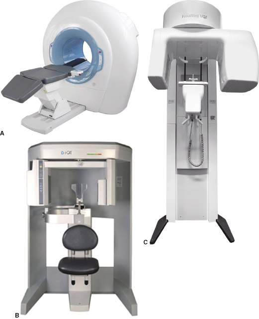
The various CBCT scanners grouped on the basis of patient positioning in the scanner are listed below. Examples are shown in Figure 2.3.
- Supine imaging position: Newtom 3G and Newtom 5G (Quantitative Radiology, Verona, Italy) and SkyView (MyRay, Cefla Dental Group, Imola, Italy)
- Sitting imaging position: i-CAT Next Generation (Imaging Sciences International, Hatfield, PA), KaVo 3D eXam (KaVo Dental GmbH, Bismarckring, Germany), 3DE Accuitomo (J. Morita, Kyoto, Japan), Scanora (Soredex, Orion Corporation, Helsinki, Finland), and Galileos® (Sirona Dental Systems, Bensheim, Germany)
- Standing imaging position: Newtom VGi (Quantitative Radiology), ProMax (Planmeca OY, Helsinki, Finland), Galileos® (Sirona Dental Systems), and AugeZIO series (Asahi Roentgen, Kyoto, Japan).
Some CBCT units offer the option to scan with the patient in either standing or sitting position; however, none offers the option of both supine and standing positions. A unit with supine imaging position is more useful in hospital settings (e.g., trauma centers) in which patients with maxillofacial trauma or multiple injuries including head injuries are tended. Scanners with supine position also are necessary for planning radiation guidance in oncology and intraoperative planning. For the purposes of orthodontic imaging and other dental applications, CBCT units with sitting or standing features are preferred for ease of accessibility. These units require less space and their configuration decreases the likelihood of claustrophobia to the patient. In addition, due to scan time of several seconds to more than half a minute, the units offering a sitting option may be less prone to movement artifacts than those in which patients have to stand.
Classification Based on Field of View (FOV)
FOV is widely used to classify CBCT machines (Table 2.2, Table 2.3, Table 2.4 and Table 2.5). As presented by Scarfe & Farman (2008), FOVs for craniofical imaging can be classified as follows:
- Localized imaging utilizes a small FOV of 5 cm or less for scanning anatomy such as of dentoalvelaor structures and the TMJ.
- Single arch imaging is performed with a FOV of 5–7 cm.
- Interarch imaging requires a FOV of approximately 7–10 cm.
- Maxillofacial imaging requires a large FOV of 10–15 cm (mandible to nasion).
- Craniofacial imaging is used for capturing the entire craniofacial structures and requires an extended FOV of 15 cm or more.
Table 2.2 Small to medium FOV CBCT units.
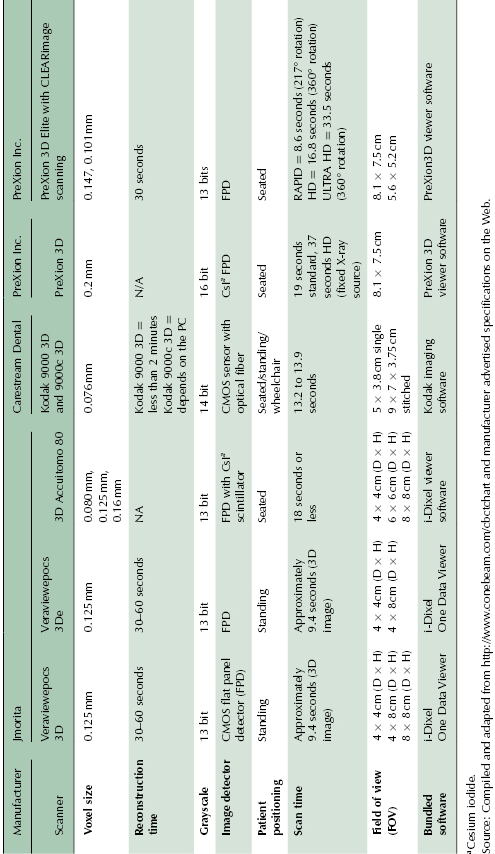
Table 2.3 Medium to large FOV CBCT units.
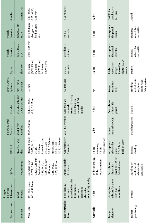
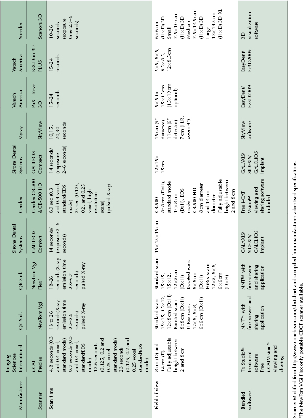
Table 2.4 Extended FOV CBCT units suitable for craniofacial imaging.
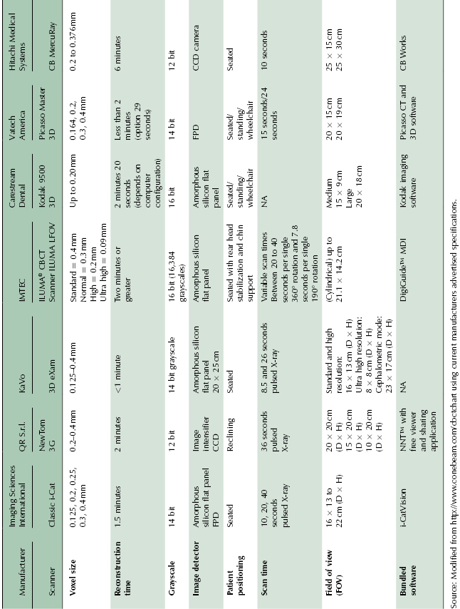
Table 2.5 CBCT units with wide range of FOV.
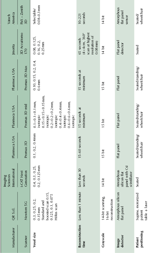
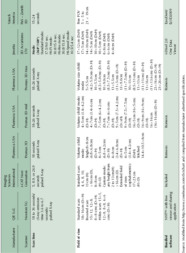
It should be noted that there is no standardized terminology for using the size of FOV for classification of the CBCT units. Extended, large, medium, and small FOV are the terms often used; however, their exact range of FOV is manufacturer defined. For example, a large FOV for one manufacturer may be of similar size to an extended FOV for another manufacturer (Table 2.2, Table 2.3, Table 2.4, and Table 2.5). FOV is usually mentioned in a range of dimensions and the volume scanned by the unit may vary from 4 × 4 cm to 25 × 30 cm depending on the FOV settings and the machine chosen. In general, a unit with large or extended FOV that also has capabilities of using smaller FOVs when desired would be preferable for orthodontic applications.
Earlier generation CBCT scanners either had fixed FOV or limited capabilities for adjusting the FOV. Currently, several manufacturers provide multiple FOV settings to incorporate flexibility in use (Table 2.2, Table 2.3, Table 2.4, and Table 2.5). Some newer units such as i-CAT Next Generation (NG), i-CAT Precise, and PaX-Reve 3D have fully adjustable FOV heights, contributing to an increase in flexibility of the units. Also, as discussed below and elsewhere (Chapter 3), FOV settings affect image quality and radiation exposure.
Other Key Attributes of CBCT Scanners
Imaging Protocols
Manufacturers currently are expanding protocols to enhance the utility and flexibility of CBCT units; however, all imaging protocols do not yield the same result in terms of radiation exposure and image quality. A clinician may choose to use specific protocols for different applications such as maxillofacial imaging, orthodontics, implant, periapical diagnosis, or endodontics.
FOV select/>
Stay updated, free dental videos. Join our Telegram channel
VIDEdental - Online dental courses


