Introduction
The purpose of this study was to propose a protocol for safe bicortical placement of mini-implants by measuring the interradicular spaces of the maxillary teeth and the bone quality.
Methods
Cone-beam computed tomography data were obtained from 50 adults. Three-dimensional reconstructions and measurements were made with SimplantPro software (Materialise, Leuven, Belgium). For each interradicular site, the bone thicknesses and interradicular distances at the planes 1.5, 3, 6, and 9 mm above the cementoenamel junction were measured. Standard bone units were defined to evaluate the influences of bone density and the different placement patterns on the stability of the mini-implants.
Results
The safe interradicular sites in the maxilla for bicortical placement of 1.5-mm-diameter mini-implants were in all planes between the first and second premolars, and between the second premolar and the first molar. The safe palatal sites were between the first and second molars, and the safe labial sites of the 9-mm plane were between the central incisors, and between the lateral incisor and the canine. The safe buccal sites of the 6- and 9-mm planes were between the first and second molars, and the safe buccal sites of the 3-, 6-, and 9-mm planes were between the canine and the first premolar. Most bone thicknesses were from 8 to 12 mm. The optimal placement angle between the second premolar and the first molar was 58°. Bicortical placement could have more standard bone units than unicortical placement in the maxilla.
Conclusions
Bicortical placement would be more stable in the maxilla. For the site between the molars, special care should be taken at a plane higher than 6 mm to prevent maxillary sinus penetration. The most favorable interradicular area in the maxilla was between the second premolar and the first molar.
Highlights
- •
Optimal bicortical placement sites and angles were measured in 3 dimensions.
- •
We defined standard bone units to evaluate bicortical implant stability.
- •
Bicortical placement would be more stable in the maxilla.
Appropriate anchorage in orthodontic treatment is important. Mini-implants have gained considerable popularity because of their low cost, effectiveness, easy clinical management, and stability. Among the factors related to mini-implant stability, alveolar bone thickness, bone density, placement a ngle, and location appear to be critical for successful placement. Adequate bone quantity at the placement site can affect the success of the mini-implants. This has prompted further research for the ideal sites and the greatest stability for mini-implants.
Bone density appears to be a key determinant for the stability of mini-implants in sites with inadequate cortical bone thickness because primary retention of mini-implants during the early stages of placement is achieved by mechanical means rather than through osseointegration. The distribution of mechanical stress occurs primarily where bone contacts the implant. Bone density influences the amount of bone in contact with the implant surface, and thus the stress can also be reduced by increasing the functional area over which the force is applied by increasing either the length or the diameter of the implant. The results of previous studies have suggested that bone of higher density might ensure a better biomechanical environment for mini-implants. Moreover, longer screw-type mini-implants could be a better choice in a jaw with low bone density. In the comparatively weak cortical bone area, stress is known to be distributed to both cancellous and cortical bone, whereas where the cortex is thick and dense, stress is centered on the cortical bone. When this is considered with the study of Hedia, showing that stress can be concentrated at the cortical bone with weak or no cancellous bone, the cancellous bone in the maxilla might have a greater influence on success than that in the mandible. Unicortical anchorage occurs when the mini-implant penetrates only 1 cortical plate, whereas with bicortical anchorage, the mini-implant is long enough to penetrate 2 cortical plates. The in-vitro experimental findings of Brettin et al showed that bicortical mini-implants provide superior anchorage resistance, reduced overall cortical bone stress, and superior stability compared with unicortical mini-implants.
Clinically, computed tomography (CT) is currently the only diagnostic imaging technique that allows for a rough determination of the structure and density of bone in the jaws. It is also an excellent tool for assessing the relative distributions of cortical and cancellous bone in an anatomic structure. In recent years, cone-beam CT (CBCT), which offers clear 3-dimensional (3D) images with small voxel size, has been widely used in orthodontics and implant dentistry for accurate surgical guidance of mini-implant placement and is a reliable tool to objectively determine site-specific bone density.
The objectives of this study were to determine the interradicular spaces between the maxillary teeth using 3D CBCT data, and to determine the optimal sites, directions, and angles for the placement of bicortical mini-implants in orthodontic treatment. Additionally, we sought to evaluate bone density and quality at common orthodontic implant sites with quantitative measurements of the simulated placement of mini-implants in the maxillary interradicular bone, and to propose a protocol for safe bicortical mini-implant placement.
Material and methods
Our sample consisted of the CBCT data from 50 adults (22 men, 28 women; ages, 18-39 years; average age, 25.7 years). All patients met the following criteria: no periodontitis or posterior arch discrepancy; posterior teeth not rotated or malformed; and no history of orthodontic treatment before the collection of the CBCT images. These subjects gave written informed consent to publish the resulting data and case details.
The images were taken with a CBCT apparatus (NewTom VGi; QR Srl, Verona, Italy) at 110 kV, 0.07 mAs, slice thickness of 0.3 mm, and pixel size of 0.3 mm. The CBCT data were saved as DICOM files. Three-dimensional reconstruction procedures and measurements were made with SimplantPro software (Materialise, Leuven, Belgium).
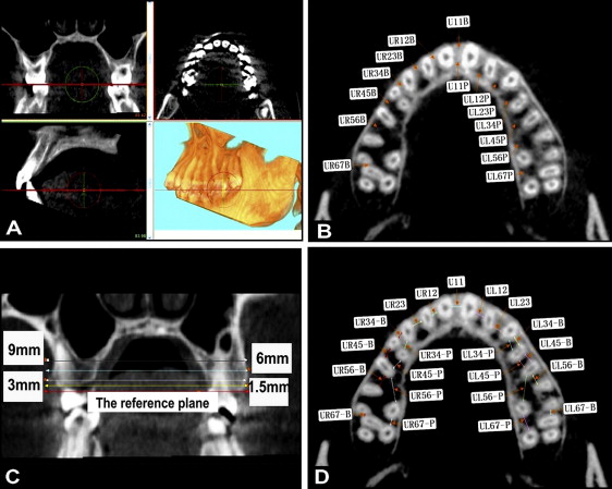
To measure the interradicular distances, the axial images were reoriented to the occlusal plane ( Fig 1 , A ), and then sequential axial plane images of 1.5, 3, 6, and 9 mm from the cementoenamel junction (CEJ) apical and parallel to the occlusal plane were constructed ( Fig 1 , B and C ). The CEJ plane, used as the reference, was defined as a plane through the midpoints of the CEJ of 2 adjacent teeth and parallel to the occlusal plane. The narrowest interradicular distances between neighboring roots were measured in each axial plane ( Fig 1 , D ). Because of the multiroot nature of the molars, the buccal and palatal root distances in the molar areas were measured individually.
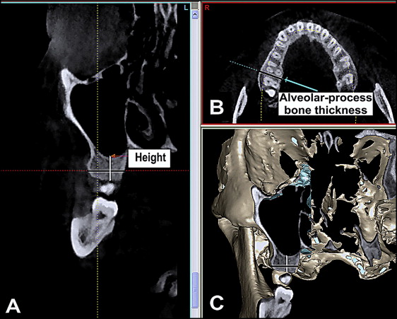
To measure the distance between the sinus floor and the CEJ of each interradicular area, a panoramic curve on the axial image was drawn, and then the shortest distance was measured on the slice images ( Fig 2 , A ). On the sequential axial plane images, the alveolar process bone thickness of each interradicular area was measured ( Fig 2 , B ).
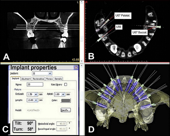
At each site, the optimal bicortical placement angle was measured in relation to the sagittal plane. In the site mesial to the first molar, the optimal placement of the mini-implant was along a line bisecting the angle of the adjacent roots. In the buccal site between the first and second molars, the optimal placement of the mini-implant was along the angle bisecting the second molar’s mesiobuccal root and that of the first molar. When the maxillary molar was rotated, unicortical placement was selected in the palatal site between the first and second molars ( U67P in Fig 3 , B ), with the optimal placement of the mini-implant along the angle bisecting the first and second molars’ palatal roots. Mini-implants with a diameter of 1.5 mm were always used in clinical practice and thus were used in the simulation for each interradicular site along the optimal angles at the different axial planes ( Fig 3 , A and D ). The angles between the mini-implants and the sagittal plane are shown in the implant properties ( Fig 3 , C ), and the mean angles were recorded.
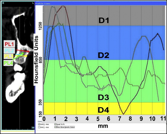
Misch and Kircos classified bone density into 5 types based on Hounsfield units (HU): D1, more than 1250 HU; D2, 1250 to 850 HU; D3, 850 to 350 HU; D4, 350 to 150 HU; and D5, less than 150 HU. In our effort to determine bone quality, we defined “standard bone units” using 1-mm-thick bone slices from the CBCT images as follows: <SPAN role=presentation tabIndex=0 id=MathJax-Element-1-Frame class=MathJax style="POSITION: relative" data-mathml='standard boneunits=(mean bone density−150)200×bone thickness’>standard boneunits=(mean bone density−150)200×bone thicknessstandard boneunits=(mean bone density−150)200×bone thickness
standard bone units = ( mean bone density − 150 ) 200 × bone thickness
. Thus, mean bone density higher than 350 HU would be rated as 1 “standard bone unit,” making a 1-mm slice of bone at a mean density of 350 HU the basis for a standard bone unit of 1. Then a 1-mm slice of D1 bone with a mean density of 1650 HU may have 7.5 standard bone units, a 1-mm slice of D2 bone with a mean density of 1050 HU may have 4.5 standard bone units, a 1-mm slice of D3 bone with a mean density of 600 HU may have 2.25 standard bone units, and a 1-mm slice of D4 bone with a mean density of 250 HU may have only 0.5 standard bone unit.
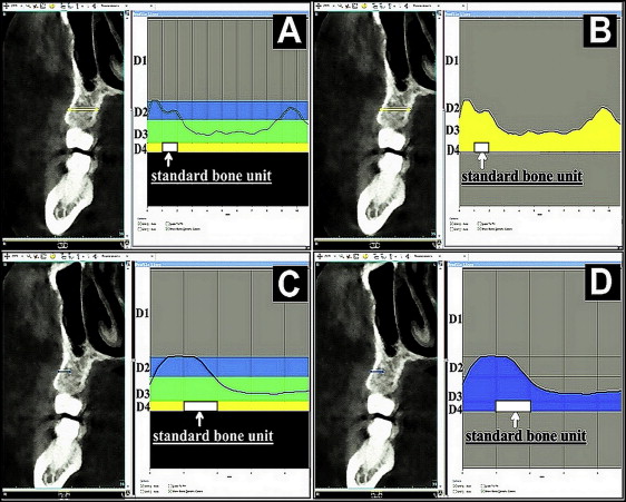
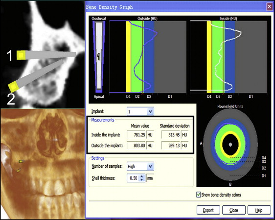
To evaluate the influence of bone density and the different placement patterns on the stability of mini-implants, the profile lines of 4 placement patterns in maxillary interradicular bone were used to visualize the intensity of the varying densities along the defined lines ( Fig 4 ). Placement patterns 1 and 3 were bicortical placements, and placement patterns 2 and 4 were unicortical placements. In the profile line list, the Hounsfield units along the created profile line are presented. The colors of the different bone density types are indicated on the graphs and facilitate the interpretation of the Hounsfield units. The profile picture was imported into Photoshop software (Adobe, San Jose, Calif) to calculate the total area between the profile line and the bottom line of the D4 bone (150 HU). The area of 1-mm D4 bone may be interpreted as 1 standard bone unit ( Fig 5 , A and C ). Then the total area was divided by the area of 1-mm D4 bone to identify the total bone units of the profile ( Fig 5 , B and D ). The bone density graph gives the mean bone density along the profile line ( Fig 6 ).
Standard bone units = ( mean bone density − 150 ) 200 × bone thickness .
Stay updated, free dental videos. Join our Telegram channel
VIDEdental - Online dental courses


