Introduction
The objective of this study was to evaluate the effect of the orientation of cone-beam computed tomography (CBCT) images on the precision and reliability of 3-dimensional cephalometric landmark identification.
Methods
Ten CBCT scans were used for manual landmark identification. Volume-rendered images were oriented by aligning the Frankfort horizontal and transorbital planes horizontally, and the midsagittal plane vertically. A total of 20 CBCT images (10 as-received and 10 oriented) were anonymized, and 3 random sets were generated for manual landmark plotting by 3 expert orthodontists. Twenty-five landmarks were identified for plotting on each anonymized image independently. Hence, a total of 60 images were marked by the orthodontists. After landmark plotting, the randomized samples were decoded and regrouped into as-received and oriented data sets for analysis and comparison. Means and standard deviations of the x-, y-, and z-axis coordinates were calculated for each landmark to measure the central tendency. Intraclass correlation coefficients were calculated to analyze the interobserver reliability of landmark plotting in the 3 axes in both situations. Paired t tests were applied on the mean Euclidean distance computed separately for each landmark to evaluate the effect of 3-dimensional image orientation.
Results
Interobserver reliability (intraclass correlation coefficient, >0.9) was excellent for all 25 landmarks for the x-, y-, and z-axes on both before and after orientation of the images. Paired t test results showed insignificant differences for the orientation of volume-rendered images for all landmarks except 3: R1 left ( P = 0.0138), sella ( P = 0.0490), and frontozygomatic left ( P = 0.0493). Also midline structures such as Bolton and nasion were plotted more consistently or precisely than bilateral structures.
Conclusions
Orientation of the CBCT image does not enhance the precision of landmark plotting if each landmark is defined properly on multiplanar reconstruction slices and rendered images, and the clinician has sufficient training. The consistency of landmark identification is influenced by their anatomic locations on the midline, bilateral, and curved structures.
Highlights
- •
This study provides insight into influence of orientation of CBCT image on 3D landmark plotting.
- •
Landmark plotting was performed by 3 observers blindly and randomly to prevent bias.
- •
Excellent interobserver reliability was obtained for as-received and oriented CBCT data sets on landmark plotting.
- •
The locations of landmarks influence the consistency of their identification in both situations.
Three-dimensional craniofacial imaging such as computed tomography (CT) and cone-beam CT (CBCT) offers great potential in diagnosis and treatment planning of complex skeletal deformities and assessment of growth and treatment effects. Conventionally, craniofacial analyses based on 2-dimensional (2D) cephalometry have several limitations: magnification, distortion, overlapping of craniofacial structures, difficulty in locating hidden anatomic structures, and so on. These limitations were also highlighted during comparisons of measurements between dry skulls and those on 2D cephalograms while searching for the anatomic truth. With the advancements in 3-dimensional (3D) imaging modalities in the last decade, these limitations of 2D analysis have been addressed to a certain extent.
Synchronal literature in this decade has emphasized the pivotal role of 3D CT and CBCT imaging modalities in the 3D cephalometric analysis. But the challenge for clinicians at present is to understand and interpret 3D imaging. Conventionally, cephalometric analysis is based on the landmark identification and plotting on 2D images. Training and familiarization with the location of landmarks on 3D images is essential because landmark identification errors are a major source of cephalometric errors. Therefore, the need for new guidelines for 3D landmark identification is warranted.
Many studies in recent years have evaluated the reliability of landmark identification on CT and CBCT data. Apart from the errors due to the lack of experience, the perceptions of the observer in localizing the anatomic landmarks on 3D images and the head orientation also may influence landmark plotting on 3D images. A few studies have evaluated the effect of head orientation in CBCT synthesized posteroanterior and lateral cephalograms and 3D CBCT imaging modality on cephalometric measurements. A significant difference was found between dry skull cephalometric measurements and CBCT synthesized lateral cephalogram measurements in different head positions, whereas the differences in measurements on 3D CBCT images were found to be statistically insignificant from dry skull measurements. Studies by Tomasi et al and Berco et al have shown statistically insignificant differences between nonoriented CBCT images and dry skulls; the data were derived using only a single skull for measurements. Similarly, Ludlow et al and Hassan et al have also shown insignificant measurement differences between nonoriented CBCT data and dry skulls with 4 and 10 linear measurements, respectively.
These studies have tried to provide insight into the effect of head orientation on the accuracy of linear measurements but not on the anatomic landmark positions in 3 dimensions with a change in orientation ( Table I ). To authenticate the accuracy of plotted landmarks, baseline data (gold standard) were required to be derived from the markings on the actual skull models for comparison. Since it is not possible to obtain gold standard measurements directly from living subjects, data can possibly be derived by repeated landmark plotting on CBCT images. The precision of landmark plotting could be influenced by the orientation of the volume-rendered image. Direct evaluation of precision and consistency of 3D landmark plotting with and without orientation has not been investigated. In the light of such data with uncertain standpoints on the effect of orientation on landmark identification, this study was conducted to evaluate the effect of orientation on the precision of 3D landmark identification vis-à-vis as-received CBCT images.
| Study | Authors | Objective | Sample size | Observers (n) | Observations per observer (n) | Landmarks (n) | Measurements (n) |
|---|---|---|---|---|---|---|---|
| 1. | Neiva et al (2014) | Landmark identification comparison between CBCT MPR and 3D reconstruction | 12 CBCTs | 3 | 3 (on 3D) + 3 (on MPR) = 6 | 28 | – |
| 2. | Tomasi et al (2011) | Influence of inclination of the object on reliability and reproducibility of CBCT measurements | 1 dry mandible | 3 | 3 (physical) + 4 (on optimal CBCT scan) + 4 (on 45° rotated CBCT scan) = 11 | – | 10 |
| 3. | Cevidanes et al (2009) | Head orientation in CBCT generated 2D cephalograms | 12 CBCTs | 3 | 4 (2 on NHP 2D projection and 2 on oriented 2D projection) | – | 50 |
| 4. | Hassan et al (2009) | Influence of patient scanning position | 8 dry skulls | 3 | 2 (physical) + 2 (on 3D) + 2 (MPR) + 2 (on lateral and PA projection) = 8 | 8 | 10 |
| 5. | Berco et al (2009) | Accuracy and reliability of 3D craniofacial measurements | 1 dry skull | 2 | 4 (physical) + 4 (on optimal CBCT scan) + 4 (on 45° rotated CBCT scan) = 12 | 17 | 29 |
| 6. | Ludlow et al (2007) | Influence of rotation on measurements made over 2D and 3D images | 30 dry skulls | 1+1+1 | 2 (physical) + 1 (physical) + (2 [on panoramic] and 2 [on 3D]) | – | 4 |
| 7. | Present study | Influence of orientation | 10 CBCTs | 3 | 1 (before orientation) + 1 (after orientation) = 2 | 25 | – |
Material and methods
Ten CBCT images were collected randomly from an orthodontic clinic database retrospectively irrespective of age, sex, and ethnicity. The ethics committee of All India Institute of Medical Sciences, New Delhi, India approved this study, and no patients were recruited for this study separately. The CBCT scans were obtained using an i-CAT next generation machine (Imaging Sciences International, Hatfield, Pa) with a field of view of 17 × 22 cm and a scan time of 26 seconds. The data were saved in DICOM (version 1.7) format with an isometric voxel size of 0.25 to 0.30 mm. CBCT scans had been taken with the subject sitting upright and in natural head position.
Three experienced orthodontists (R.B., S.K., S.C.) were asked to plot the landmarks on the CBCT images and were called O1, O2, and O3. Furthermore, 2 observers (A.G., V.S.) separately were asked to perform orientations of the CBCT images and randomization of the data for blind marking for the experiment. The observer who had performed the orientations was called O4, and the observer who had randomized the data for blind marking was called O5. Observer O5 generated 3 random sets of CBCT data referred to as SI, SII, and SIII for landmark plotting of the 3 observers O1, O2, and O3.
Twenty-five commonly used cephalometric landmarks were selected, and operational definitions of each landmark in the 3 planes (axial/xy plane, coronal/xz plane, and sagittal/yz plane) were derived. In addition to the cross-sectional slices, 3D volume-rendered images were also used to confirm landmark positions. Three axes were defined: x-axis in the right-left direction, y-axis in the anteroposterior direction, and z-axis in the inferior-superior direction. The 3 orthodontists who participated in the study were familiarized with each landmark and mutually agreed on the definitions of each landmark in 3 dimensions. They practiced on 5 anonymized CBCT images. Any ambiguity in locating landmarks was resolved through mutual discussion, and the landmark definitions were refined with the consensus of the expert orthodontists. It was decided to plot 11 landmarks in volume-rendered images directly and confirm them on multiplanar reconstruction slices; the remaining 14 landmarks were plotted in reverse order ( Table II ).
| Landmark | Abbreviation | Definition on skull | Sagittal slice | Axial slice | Coronal slice | Remarks | |
|---|---|---|---|---|---|---|---|
| 1. | Nasion | N | Most anterior point of the frontonasal suture in the midsagittal plane | Anterior-most point | Middle-anterior most point on the anterior contour | Middle point | Plotted on 3D volumetric data and confirmed on MPR views |
| 2. | Orbitale left | Or L | The lowest point in the inferior margin of the left orbit | Anterior-superior most point | – | – | Plotted on 3D volumetric data and confirmed on MPR views |
| 3. | Orbitale right | Or R | The lowest point in the inferior margin of the right orbit | Anterior-superior most point | – | – | Plotted on 3D volumetric data and confirmed on MPR views |
| 4. | A-point | A-point | The point at the deepest midline concavity on the maxilla between the anterior nasal spine and the dental alveolus | Posterior-most point | Middle-anterior most point on the anterior contour | Middle point determined by the sagittal and axial slices | Plotted through MPR views and confirmed on 3D volumetric data |
| 5. | Anterior nasal spine | ANS | Most anterior midpoint of the anterior nasal spine of maxilla | Most anterior point | Anterior point and middle point | Middle point | Plotted through MPR views and confirmed on 3D volumetric data |
| 6. | Posterior nasal spine | PNS | The sharp posterior extremity of the nasal crest of the hard palate | Most posterior point | Posterior point and midpoint | – | Plotted through MPR views and confirmed on 3D volumetric data |
| 7. | B-point | B-point | Most posterior point in the concavity along the anterior border of the mandibular symphysis | Posterior-most point | Middle-anterior most point on the anterior contour | Middle point determined by the sagittal and axial slices | Plotted through MPR views and confirmed on 3D volumetric data |
| 8. | Pogonion | Pog/Pg | Most anterior point on mandibular symphysis | Anterior-most point | Middle-anterior-most point on the anterior contour | Middle point determined by the sagittal and axial slices | Plotted through MPR views and confirmed on 3D volumetric data |
| 9. | Menton | Me | Most inferior point on the mandibular symphysis | Inferior-most point | Middle most point | Middle inferior-most point | Plotted through MPR views and confirmed on 3D volumetric data |
| 10. | Gnathion | Gn | Midpoint of the curvature of pogonion and menton | Anterior-inferior most point | Middle-anterior most point | Middle inferior-most point | Plotted through MPR views and confirmed on 3D volumetric data |
| 11. | Gonion left | Go L | Most inferior and posterior point on left mandibular corpus | Inferior and posterior most point | Posterior most point | Inferior-most point | Plotted on 3D volumetric data and confirmed on MPR views |
| 12. | Gonion right | Go R | Most inferior and posterior point on right mandibular corpus | Inferior and posterior most point | Posterior most point | Inferior-most point | Plotted on 3D volumetric data and confirmed on MPR views |
| 13. | Condylion left | Co L | Most superior point on the left mandibular condyle | Superior-most point | Midpoint determined by the sagittal and coronal slices | Middle superior-most point | Plotted through MPR views and confirmed on 3D volumetric data |
| 14. | Condylion right | Co R | Most superior point on the right mandibular condyle | Superior-most point | Midpoint determined by the sagittal and coronal slices | Middle superior-most point | Plotted through MPR views and confirmed on 3D volumetric data |
| 15. | R1 left | R1 L | The deepest point on the curve of the anterior border of the left ramus | Deepest point | Anterior point | – | Plotted on 3D volumetric data and confirmed on MPR views |
| 16. | R1 right | R1 R | The deepest point on the curve of the anterior border of the right ramus | Deepest point | Anterior point | – | Plotted on 3D volumetric data and confirmed on MPR views |
| 17. | Sella | S | Midpoint of sella turcica | Middle point of the pituitary fossa | Middle point of the anteroposterior and lateral width of the pituitary fossa | Middle point of the lateral width of the fossa determined by the sagittal and axial slices | Plotted through MPR views and confirmed on 3D volumetric data |
| 18. | Basion | B | The most anterior point on the anterior margin of the foramen magnum in the midsagittal plane | Inferior-posterior most point | Anterior-most point | Middle point | Plotted through MPR views and confirmed on 3D volumetric data |
| 19. | Zygomatic point left | Zy L | The most lateral point on the left outline of left zygomatic arch | – | Anterior lateral point | Most lateral and superior point | Plotted on 3D volumetric data and confirmed on MPR views |
| 20. | Zygomatic point right | Zy R | The most lateral point on the right outline of right zygomatic arch | – | Anterior lateral point | Most lateral and superior point | Plotted on 3D volumetric data and confirmed on MPR views |
| 21. | Frontozygomatic left | Fz L | The most medial and anterior point of left frontozygomatic suture at the level of the lateral orbital rim | Most anterior | Most anterior | Medial point | Plotted on 3D volumetric data and confirmed on MPR views |
| 22. | Frontozygomatic right | Fz R | The most medial and anterior point of right frontozygomatic suture at the level of the lateral orbital rim | Most anterior | Most anterior | Medial point | Plotted on 3D volumetric data and confirmed on MPR views |
| 23. | Jugal point left | J L | The deepest midpoint of left jugal process of maxilla | Inferior-most point | – | Deepest point | Plotted through MPR views and confirmed on 3D volumetric data |
| 24. | Jugal point right | J R | The deepest midpoint of right jugal process of maxilla | Inferior-most point | – | Deepest point | Plotted through MPR views and confirmed on 3D volumetric data |
| 25. | Bolton | Bo | The most posterior point of foramen magnum in midsagittal plane | Anterior point of posterior border of foraman magnum | Mid and posterior most point | Middle point | Plotted through MPR views and confirmed on 3D volumetric data |
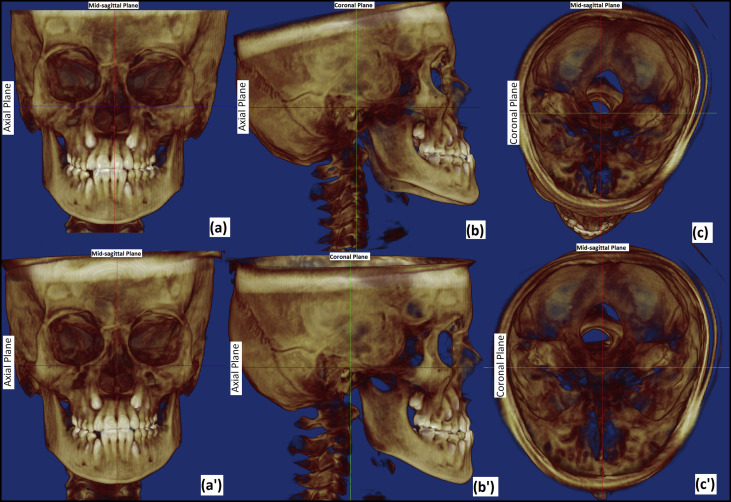
For the purpose of orientation, DICOM data were imported into Dolphin 3D software (version 11.5; Dolphin Imaging and Management Systems, Chatsworth, Calif). Volume-rendered images were oriented by aligning the Frankfort horizontal plane and the transorbital plane horizontally, and the midsagittal plane vertical ( Fig 1 ) by an observer (O4), who was not involved in landmark plotting. After satisfactory orientation, new DICOM image slices/series were saved. A total data set of 20 CBCT images (10 as-received and 10 after orientation) was thus created. These data sets were then anonymized for blind landmark plotting using Mimics software (Materialise, Leuven, Belgium) by the same observer (O4). To prevent bias, all as-received and oriented datasets were kept in 1 folder and renamed randomly with numbers from 1 to 20 in the order of plotting by an observer (O5) who had not performed the orientation of the CBCT images. Three random sets (SI, SII, SIII) of data were generated in the same manner for each of the 3 observers (O1, O2, O3). Hence, the observers were neither aware of the orientation of the CBCT data sets nor of the order of the CBCT images for the other observers.
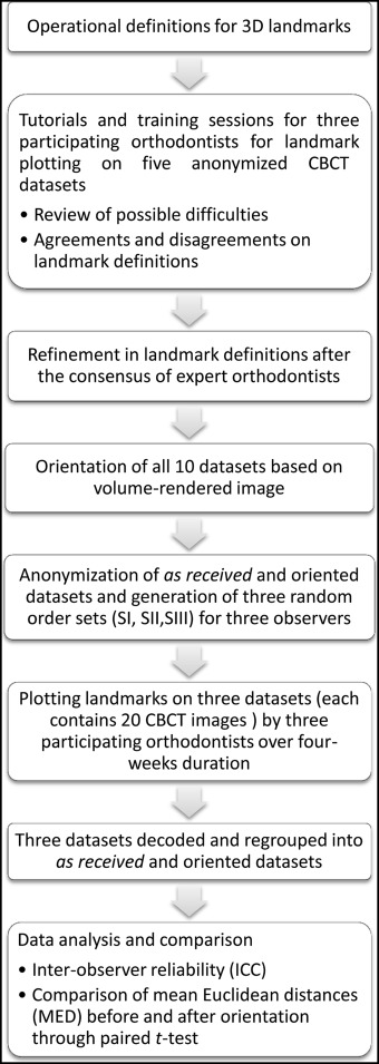
Three observers (O1, O2, O3) independently plotted 25 cephalometric landmarks on 20 CBCT images over 4 weeks. After landmark plotting, the randomized samples were decoded and regrouped into as-received and oriented data sets for analysis and comparison. The adopted methodology of landmark plotting is depicted in Figure 2 . Three-dimensional coordinates (x, y, and z) of each landmark from all 20 data sets were exported into Excel (Microsoft, Redmond, Wash) sheets for the as-received and oriented datasets.
The mean of all 3 observers marking for each coordinate of the landmarks was used as the centroid for that landmark. Three-dimensional mean Euclidean distances (MED), mean deviations from centroid, and standard deviations were calculated separately for statistical analysis. The centroid of the 3 observers’ markings for each landmark was considered as the gold standard. The mean of the Euclidean distances from the centroid of the observers’ markings to each observer’s marking represented the error in the detection of that landmark. The variations of MED before and after orientation of the 3D images were analyzed. MED analyzed the overall error (rather than in each axis) in landmark identification. Therefore, the mean deviation was computed to analyze the variation in each axis of all landmarks. Standard deviations represented the variations among all samples of each landmark. The standard deviations were computed for both MED and mean deviation to demonstrate the distribution of errors over the number of samples.
MED was calculated as shown in Figure 3 . To obtain the MED, following steps were carried out.
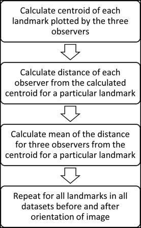
Step 1: A centroid was calculated with the 3D coordinates of all 3 observers for every landmark in each data set
C e n t r o i d ( C L ) = ( O x 1 + O x 2 + O x 3 3 , O y 1 + O y 2 + O y 3 3 , O z 1 + O z 2 + O z 3 3 )
where C L ( L is any of the 25 landmarks) represents the coordinate of the centroid, and Oij
O j i
( j = x, y, z; i = first, second, and third observers) is the coordinates in x-, y- and z-axes for the 3 observers, respectively.
Step 2: Euclidean distance for each observer from the centroid for all 3 observers was calculated by using the following Euclidean distance formula.
D i s t a n c e ( D L i ) = ( C L x − O x i ) 2 + ( C L y − O y i ) 2 + ( C L z − O z i ) 2
where DiL
D L i
is the Euclidean distance for each observer from the centroid ( i = first, second, and third observers), and L is any of the 25 landmarks.
C L = ( C Lx , C Ly , C Lz ); C Lx , C Ly and C Lz are x-, y- and z-axes coordinates of the centroid for the L landmark, and Oij
O j i
( j = x, y, z; i = first, second, and third observers) is the coordinates in the x-, y- and z-axes for the observers, respectively.
Step 3: The mean distance of the 3 observers was calculated separately for every landmark for each of the 10 data sets and called MED.
M e a n E u c l i d e a n D i s t a n c e ( M E D L s ) = D L 1 + D L 2 + D L 3 3
where MEDsL
M E D L s
( L is any of the 25 landmarks; S [sample] = 1, 2, 3, …, 10 for the data sets) is the MED for every landmark of each data set.
Step 4: Similarly, MED was calculated for all 25 landmarks in the 10 data sets obtained after orientation of the images.
Mean differences and standard errors were calculated on the basis of MED for the 25 landmarks before and after orientation of the images.
M e a n d i f f e r e n c e ( M L ) = | ∑ S = 1 10 ( M E D L S ) B O − ∑ S = 1 10 ( M E D L S ) A O 10 |
Stay updated, free dental videos. Join our Telegram channel
VIDEdental - Online dental courses


