Introduction
The purpose of this study was to present and validate a novel semiautomated method for 3-dimensional evaluation of the temporomandibular joint (TMJ) space and condylar and articular shapes using cone-beam computed tomographic data.
Methods
The protocol for 3-dimensional analysis with the Checkpoint software (Stratovan, Davis, Calif) was established by analyzing cone-beam computed tomographic images of 14 TMJs representing a range of TMJ shape variations. Upon establishment of the novel method, analysis of 5 TMJs was further repeated by several investigators to assess the reliability of the analysis.
Results
Principal components analysis identified 3 key components that characterized how the condylar head shape varied among the 14 TMJs. Principal component analysis allowed determination of the minimum number of landmarks or patch density to define the shape variability in this sample. Average errors of landmark placement ranged from 1.15% to 3.65%, and none of the 121 landmarks showed significant average errors equal to or greater than 5%. Thus, the mean intraobserver difference was small and within the clinically accepted margin of error. Interobserver error was not significantly greater than intraobserver error, indicating that this is a reliable methodology.
Conclusions
This novel semiautomatic method is a reliable tool for the 3-dimensional analysis of the TMJ including both the form and the space between the articular eminence and the condylar head.
Highlights
- •
We developed a program to 3-dimensionally define the temporomandibular joint.
- •
We determined the optimal patch density for this semiautomated analysis.
- •
We demonstrated reliability on a subset of 5 temporomandibular joints.
- •
Average error of landmark placement ranged from 1.15% to 3.65%.
- •
We evaluated principal components with 14 condyles and determined their average shape.
Conventional 2-dimensional radiographs have major drawbacks in the assessment of condylar position and morphology because of overlapping anatomic structures and inherent distortion in 2-dimensional imaging of a 3-dimensional (3D) structure, as well as magnification errors. Furthermore, with conventional radiography and tomography, it is difficult to reproduce the x-ray beam projection for follow-up radiography; this is crucial for long-term evaluation of the temporomandibular joint (TMJ). Condylar position changes should be analyzed in 3 dimensions; to achieve this with conventional radiographs, multiple views are required, such as combining submentovertex radiographs and axially corrected sagittal and coronal tomography. Computed tomography provides far superior imaging of the hard tissues of the TMJ, and 1 imaging sequence provides the necessary information, but the increased radiation exposure and high cost have limited its application. Although magnetic resonance imaging provides images of both soft and hard tissues without exposing patients to radiation, high cost and a long scanning time makes it less accessible.
Cone-beam computed tomography (CBCT) has overcome many shortcomings of the aforementioned imaging techniques. Hilgers et al found that CBCT images are highly accurate compared with direct anatomic measurements, whereas measurements made with conventional radiographs are significantly greater than the anatomic truth. A similar finding was reported by Honey et al when comparing the diagnostic accuracy of CBCT with that of panoramic film and linear tomograms for detection of simulated condylar defects. CBCT provides accurate 3D imaging of the TMJ using a lower radiation dose and at a lower cost compared with conventional computed tomography. Hence, CBCT has been used extensively as the method of choice to evaluate changes in condylar position and morphology.
Although 3D visual data are readily available with CBCT, perhaps the most common method of TMJ analysis with CBCT data now is to make linear and angular measurements in the multiplanar cross-sections of the joint. This approach, although proven accurate, fails to take full advantage of the CBCT data because it converts the 3D data into a series of 2-dimensional cross-sectional images.
Recently, superimpositions of reconstructed images from CBCT data combined with color-mapping techniques have enabled 3D visualization of the skeletal changes after orthognathic surgery, and this technique has been applied to monitor condylar position changes. A similar method has been used to quantify the amount of resorption in TMJ osteoarthritis. Other studies have taken an alternative approach and focused on the condylar volume. However, currently, there are no methods that allow 3D evaluation of the glenoid fossa and the condyle as an anatomic unit to determine the relationship between the osseous components of the TMJ.
The purpose of this study was to present and validate a novel semiautomated method for 3D evaluation of the TMJ using CBCT data. The specific aims were to introduce a novel semiautomated 3D analysis of the TMJ using CBCT data and to determine its intraoperator and interoperator reliability. The hypothesis was that the semiautomated 3D analysis of the TMJ space and shape has high intraobserver and interobserver reliability. Another specific aim was to determine the minimum number of landmarks that define the range of shape variability of the condyle and the articular eminence in this sample using principal components analysis (PCA).
Material and methods
To establish the new protocol for the 3D analysis of the TMJ, CBCT images of 14 TMJs representing a broad range of TMJ shapes that might be clinically expected were selected from a pool of available data. The patients (9 female, 5 male) had an average age of 21.8 ± 6.04 years and an age range of 10 to 30 years. Of those, 5 TMJs were randomly selected to investigate the reproducibility of the novel method. All CBCT scans were taken by the same radiographic technician using the same scanner with the same settings and techniques. CBCT scans that were not taken in habitual maximum intercuspation and with the condyles visibly out of the fossae were excluded from the study. The research protocol was approved by the Human Research Committee at the University of California San Francisco (number 10-00564).
All scans were taken with the i-CAT Cone Beam 3D Imaging System (Imaging Sciences International, Hatfield, Pa) with the subject in an upright sitting position with the Frankfort horizontal plane parallel to the floor. The scanning settings for the CBCT machine were as follows: 13 × 13-cm field of view (voxel size, 0.250 mm) or extended 16 × 16-cm field of view (voxel size, 0.450 mm) when a patient’s craniofacial structures including nasion and menton could not be captured with the smaller field of view, 120-kV(p) tube voltage, tube current of 18.45 to 47.74 mA, and 20-second scan time for the 13 × 13-cm field-of-view scans and 40-second scan time for the 16 × 16-cm field-of-view scans. Data from the CBCT were exported in DICOM format.
Checkpoint software (Stratovan, Davis, Calif) was used for the 3D TMJ space and shape analysis, following the step-by-step protocol outlined below.
- 1.
Isolation of the region of interest. DICOM data of the patient’s head scan were imported. The right and left condyle-fossa units were isolated using the cropping tool by dragging the cropping lines, which appeared as blue dashed lines in each slice window ( Fig 1 ). The cropped volume was subsequently saved and exported.
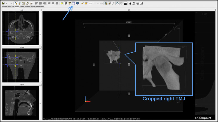
Fig 1 Cropped volume isolating the right condyle-fossa unit. - 2.
Adjustment of contrast, brightness, and isovalue. The cropped condyle-fossa unit was loaded, and the contrast and brightness of the scan were adjusted until the bony structures were well visualized. Next, the isovalue on the data histogram was adjusted to select an isosurface, seen in the 3D view and shown as a red outline in the planar windows, that best represented the cortical outlines of the condyle and the fossa.
- 3.
Orientation of the TMJ volume. The TMJ volume was oriented by moving the avatar (crosshairs) in the coronal slice where the condyle was widest mediolaterally, and by dragging over the slice rotation handles (yellow squares) so that in the axial view the horizontal line of the avatar equaled the long axis of the condyle ( Fig 2 ).
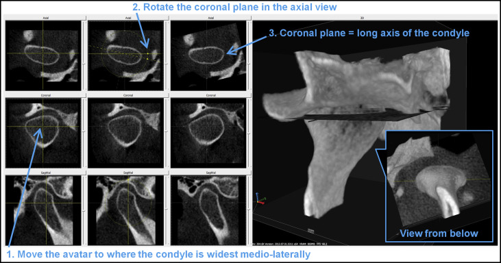
Fig 2 Oriented TMJ along the long axis of the condyle. - 4.
Control landmarks and placement. The joint landmark primitive was added on the posterior surface of the condyle. The joint primitive contains 3 control landmarks that act as “anchor points” that must be manually placed on the surface of the condyle. The yellow point was moved to the lateral pole of the condyle, and the sagittal plane was used to assist in identifying the most prominent lateral contour of the condyle ( Fig 3 ; Table I ). The red point was moved to the medial pole of the condyle, and the sagittal plane was similarly used to confirm the most prominent medial contour of the condyle ( Fig 4 ; Table I ). The white point was on the sagittal plane that is equidistant from the lateral and medial poles. To achieve this, the “align avatar to joint” option followed by the “snap condyle white landmark to sagittal slice” option was used. Finally, on the sagittal slice window, the white point was moved to the posterior aspect of the condyle where the cortication tapers to an even thickness ( Fig 5 ; Table I ).
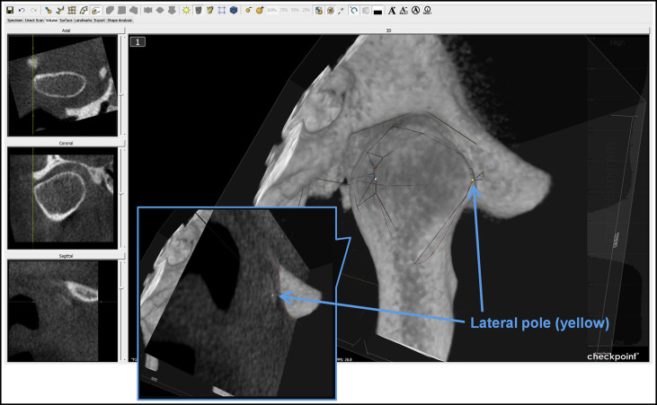
Fig 3 Yellow point placed on the lateral pole of the condyle.Table IDefinitions of the 3 condylar anchor pointsAnchor point Landmark Description Yellow Lateral pole Most prominent point on the lateral contour of mandibular condyle Red Medial pole Most prominent point on the medial contour of mandibular condyle White Posterior point Point on the posterior contour of the condyle where the cortication tapers to an even thickness 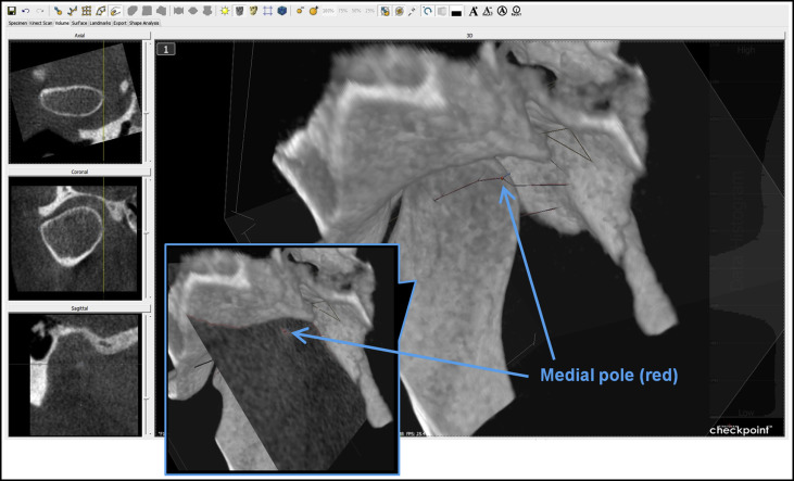
Fig 4 Red point placed on the medial pole of the condyle.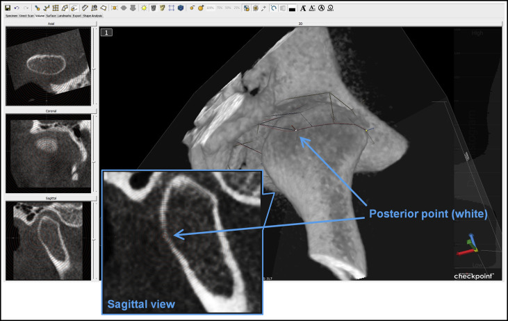
Fig 5 White point placed on the posterior contour of the condyle. - 5.
Adjustment of the semilandmarks. The aforementioned 3 control points together constituted an “equator” around the condylar head and served as the foundation for the remaining semilandmarks. Semilandmarks of a chosen density or number of points over a given area (5 × 5, 7 × 7, 9 × 9, and so on) were then automatically placed along the condyle surface using the volume data ( Fig 6 ). First, placement of each semilandmark on the condyle was reviewed one by one and adjusted if needed by dragging the point in a slice window until all semilandmarks were correctly placed on the condyle. The movement of each semilandmark was restricted to the long dotted line perpendicular to the surface.
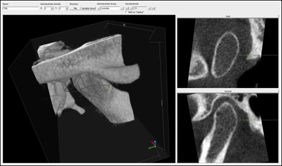
Fig 6 Automatically placed semilandmarks (density of 7 × 7) on the condyle.
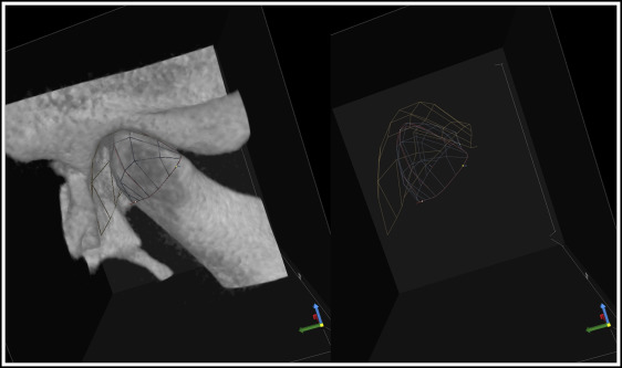
Subsequently, semilandmarks that were automatically placed on the opposing fossa surface were reviewed and adjusted. Any fossa semilandmarks that were nonexistent because of the absence of an opposing fossa wall or highly variable from being placed directly over orifices, for example, were marked as “missing” and excluded from the analysis. Finalized fossa semilandmarks and all landmarks on the condyle-fossa ( Fig 7 ) were reviewed in the volumetric view before proceeding with data analysis.
Stratovan Checkpoint software allows the user to select different patch densities (number of semilandmarks), ranging from 5 × 5 to 103 × 103, to place over the structure of interest to capture its shape. In general, lower patch densities will capture less shape variation, but there will be a point where adding more landmarks provides no additional morphologic information. As the points become clustered together, closely positioned landmarks give mostly redundant information, marginally contributing to the overall 3D information. Additionally, each additional landmark adds 3 data observations to each subject (x, y, and z coordinates), so that larger data sets will be increasingly computationally intensive, and the number of observations can far outnumber the number of subjects in a sample.
To determine which patch density can most effectively capture the shapes of the TMJ condyles and fossae, and, therefore, the joint space, 14 TMJs representing a range of TMJ shape changes were used. Each TMJ was analyzed by the steps previously described using the following densities: (1) 5 × 5, or 25 landmarks; (2) 7 × 7, or 49 landmarks; (3) 9 × 9, or 81 landmarks; (4) 11 × 11, or 121 landmarks; and (5) 13 × 13, or 169 landmarks, and all 5 patches for a given TMJ were placed directly over one another by aligning each patch at the same 3 “anchor points.”
PCA was applied to the condyle landmark coordinates for the 5 groups of different patch densities (5 × 5, 7 × 7, 9 × 9, 11 × 11, and 13 × 13). Each group consisted of landmark data from the same 14 TMJs that represented the range of shape variations that one may expect in a condyle. Using the “generalized Procrustes analysis” function, the landmark data for each of the 5 groups were first subjected to Procrustes superimposition, which translated, rotated, and scaled all landmark configurations to remove the size, position, and orientation data so that only shape information remained. Data were exported from Checkpoint, and using the geomorph package for R, all semilandmarks were slid into their most homologous positions by minimizing bending energy between specimens before the multivariate analyses. Subsequently, MorphoJ was used to perform the PCA, which analyzed the shape variance within a set of data, in this case, the 3D coordinates of condyle landmarks, and reduced the data set to a few dimensions that represented most of the variations in the data set. Applying PCA to each group helped to identify the lowest patch density that demonstrated a similar shape variance as the higher densities. In PCA, shape variance was described in terms of principal component vectors, where the first principal component accounted for the largest possible shape variance, and each succeeding component had the highest variability possible under the constraint to which it was orthogonal and, therefore, unrelated to the preceding component. The focus was placed on principal components that explained at least 10% of the total shape variance ( Table II ). To visualize the shape variation along the major principal component axes, landmark configurations representing the maxima and minima of the first 3 principal component axes were calculated by multiplying the principal components’ coefficients by the desired magnitude of shape change and adding that to the consensus configuration.


