Introduction
In this study, we investigated the landmark identification errors on cone-beam computed tomography (CBCT)-derived cephalograms and conventional digital cephalograms.
Methods
Twenty patients who had both a CBCT-derived cephalogram and a conventional digital cephalogram were recruited. Twenty commonly used lateral cephalometric landmarks and 2 fiducial points were identified on each cephalogram by 11 observers at 2 time points. The mean positions of the landmarks identified by all observers were used as the best estimate to calculate the landmark identification errors. In addition to univariate analysis, regression analysis of landmark identification errors was conducted for identifying the predicting variables of the observed landmark identification errors. To properly handle the multilayer correlations among the clustered observations, a marginal multiple linear regression model was fitted to our correlated data by using the well-known generalized estimating equations method. In addition to image modality, many variables potentially affecting landmark identification errors were considered, including location and characteristics of the landmark, seniority of the observer, and patient information (sex, age, metallic dental restorations, and facial asymmetry).
Results
Image modality was not the significant variable in the final generalized estimating equations model. The regression coefficient estimates of the significant landmarks for the overall identification error ranged from −0.99 (Or) to 1.42 mm (Ba). The difficulty of identifying landmarks on structural images with multiple overlapping—eg, Or, U1R, L1R, Po, Ba, UMo, and LMo—increased the identification error by 1.17 mm. In the CBCT modality, the identification errors significantly decreased at Ba (−0.76 mm).
Conclusions
The overall landmark identification errors on CBCT-derived cephalograms were comparable to those on conventional digital cephalograms, and Ba was more reliable on CBCT-derived cephalograms.
Conventional 2-dimensional (2D) cephalometric analyses have been used for decades to analyze dentofacial structures and evaluate growth and treatment outcomes. Despite inherent limitations such as distortion, superimposition of craniofacial structures, and differential magnifications of bilateral structures that cause difficulties in landmark identification and resulting measurement errors, conventional cephalometry remains the mainstay for evaluating craniofacial patterns.
Cone-beam computed tomography (CBCT) has become increasingly popular and has benefits in patients with craniofacial anomalies. CBCT provides tomographic views and volumetric reconstructions to capture the true 3-dimensional (3D) morphology of craniofacial structures just as multi-slice computed tomography, but CBCT has reduced acquisition time, radiation dose, and costs compared with multi-slice computed tomography. More-over, 2D images, including panoramic, lateral, and posteroanterior views, can be generated from 3D CBCT volume images. Although replacement of conventional 2D radiographs with 3D imaging appears to be a trend, CBCT is not suitable for regular, daily orthodontic patients because of its higher radiation dose than conventional radiography. The lack of 3D standard population norms has also restricted CBCT from routine orthodontic use. Since normative data for 3D CBCT volumes and new 3D paradigms are yet to be determined, it is important to evaluate the correspondence between CBCT and conventional radiography during this tran-sitional period. If CBCT-derived cephalograms prove to be equivalent to conventional cephalograms, the radiation exposure associated with conventional radiography can be eliminated in patients for whom a CBCT scan is required for 3D imaging.
Inconsistency in landmark identification is the main source of errors in cephalometric measurements. There are extensive studies on landmark identification errors for conventional cephalograms, but few studies for CBCT images. It was reported that multi-planer reconstruction displays of CBCT volume images are more precise compared with conventional cephalograms, especially for bilateral landmarks such as condylion, gonion, and orbitale. Another study reported that the reproducibility of measurements on conventional cephalograms was higher compared with those on 3D models of the same skull. Actually, landmark identification with 3D cephalometry requires more time to carefully select the best slice for landmark identification on coronal, sagittal, and axial views. Previous studies suggested that measurements taken from CBCT-derived cephalograms are comparable with those from conventional digital cephalograms in vitro and in vivo. Moreover, some landmarks on CBCT-derived cephalograms might be identified more easily than those on conventional digital cephalograms, probably because of greater differences in contrast. In addition to the characteristics of the landmarks themselves, many variables potentially affecting landmark identification errors on CBCT-derived cephalograms still have not been fully investigated. The aim of this study was to comprehensively evaluate whether landmark identification errors on CBCT-derived cephalograms are comparable with those on conventional digital cephalograms.
Material and methods
Records of 20 orthodontic patients, aged 18 to 26 years, who had both a conventional lateral cephalogram and a 22-cm CBCT scan available, were randomly selected and used in this study. Six subjects had metallic dental restorations, and 14 subjects were diagnosed with facial asymmetry with a chin deviation of ≥3.5 mm measured on the posteroanterior cephalogram. The settings used for the conventional digital lateral cephalograms by a storage-phosphor imaging system were 81 kVp, 12 mA, and 1.0 to 1.6 seconds on an Orthoceph (OC100; Imaging Division, Instrumentarium, Tuusula, Finland) with a 24 × 30-cm photo-stimulable phosphor plate, (MD 30; Agfa, Mortsel, Belgium) as the detector for image capture. The plate was scanned and digitized at 223 dots per inch. Conventional cephalometric images were exported from proprietary software, saved in JPEG format, and then imported into the cephalometric analysis software, Winceph (version 8.0; Rise, Sendai, Japan) for subsequent assessment.
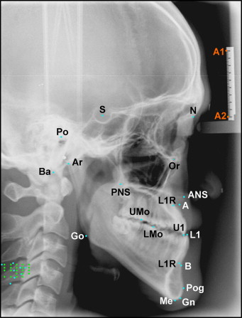
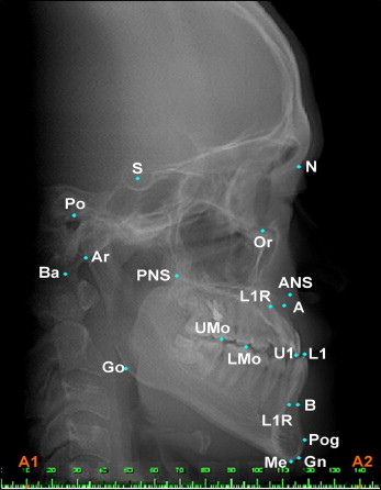
Settings used for the CBCT scans were 120 kVp, 47.74 mA, and 40 seconds with an extended height mode (22 cm) on an i-Cat CBCT scanner (Imaging Sciences International, Hatfield, Pa) with an isotropic 0.4-mm voxel size for the CBCT image. The 3D volume images were reoriented to align the midsagittal plane vertically, the Frankfort plane horizontally from the sagittal view, and the transporionic line horizontally from the frontal view. Finally, lateral cephalograms were constructed from the 3D CBCT scans by orthogonal projections, saved in JPEG format, and imported to Winceph for subsequent display and analysis. Conventional digital cephalograms were calibrated by using 2 reference points (A1 and A2) on a radiographic image of an aluminum ruler, which was attached to the cephalostat and shown in the upper left corner of the image ( Fig 1 ). The reference points were subsequently used as fiducial points to construct an x- and y-coordinate system with the origin at A1. CBCT-derived cephalograms were also calibrated by using a pair of points as fiducial points for constructing an x- and y-coordinate system ( Fig 2 ).
Eleven orthodontic residents identified 20 commonly used landmarks and the fiducial points on conventional digital and CBCT-derived cephalograms. Definitions of these cephalometric landmarks are given in Table I . All observers had similar orthodontic training backgrounds and agreed on the definitions of the landmarks. The observers were asked to zoom conventional cephalograms to 150% and CBCT-derived cephalograms to 200% before landmark identification. This process could help the observer delineate the radiographic complexity but did not compromise the image resolution. Image enhancement by fine tuning the brightness and contrast options was also allowed for better visualization of the landmarks.
| Landmark | Definition |
|---|---|
| S | Center of sella turcica |
| N | Most anterior point on frontonasal suture in the midsagittal plane |
| Or | Most inferior point on the lower border of the orbit |
| ANS | Anterior tip of the nasal spine |
| PNS | Most posterior point on the bony hard palate |
| A | Deepest point on the curve of bone between the ANS and the dental alveolus |
| B | Deepest point on the contour of the alveolar projection between the most superior point on the alveolar bone overlying the mandibular incisors and pogonion |
| Pog | Most anterior point on the symphysis of the mandible |
| Gn | Point on the chin determined by bisecting the angle formed by the facial and mandibular planes |
| Me | Most inferior point on the symphysis of the mandible |
| Go | Point on the curvature of the mandiblular angle located by bisecting the angle formed by lines tangent to the posterior ramus and the inferior border of mandible |
| Ar | Junction of the posterior ramus plane and the superstructure of the temporal bone |
| Po | Most superior point of the external acoustic meatus |
| Ba | Lowest point on the anterior rim of the foramen magnum |
| U1 | Incisal tip of the most anterior maxillary central incisor |
| U1R | The root apex of the most anterior maxillary central incisor |
| UMo | Most occlusal point on the buccal groove of the maxillary first molar |
| L1 | Incisor tip of the most anterior mandibular central incisor |
| L1R | The root apex of the most anterior mandibular central incisor |
| LMo | Most occlusal point on the buccal groove of the mandibular first molar |
For both conventional and CBCT-derived cephalograms, all observers identified the landmarks at 2 time points. The time interval between the 2 sessions was 2 weeks. The x- and y-coordinates of each landmark on the images were exported and saved for subsequent analyses. For each of the 20 landmarks, the mean x- and y-coordinates from all 11 observers were defined as the best estimates. Then the landmark identification error was expressed as a measurement in millimeters by calculating the distance of each observer’s identification from the best estimate. In addition, their horizontal and vertical components were expressed by calculating differences in the x- and y-coordinates from those of the best estimates.
Statistical analysis
Statistical analyses were performed wtih SAS software (version 9.1.3; SAS Institute, Cary, NC). A 2-sided P value ≤0.05 was considered statistically significant. The dependent variable was the landmark identification error, defined by the distance of each observer’s identification from the best estimate in millimeters. Specifically, the data of landmark identification errors consisted of the identification errors of the 11 residents, at 20 cephalometric landmarks, on 20 patients, in 2 imaging modes, and at 2 time points. This data set had a complicated correlation structure among the clustered observations.
In addition to univariate analysis, regression analysis of landmark identification errors was conducted for identifying the predicting variables of the observed landmark identification errors. To properly handle the multilayer correlations among the clustered observations, a marginal multiple linear regression model was fitted to our correlated data by using the well-known generalized estimating equations method. This estimation method was originally developed in the 1980s and has become popular for analyzing correlated data since 2000 because of the availability of statistical programs. Technically, it helped us to obtain consistent estimates of the standard errors for the estimated regression coefficients from the correlated data so that we could make consistent inferences on the regression coefficients based on the correct P values. In this generalized estimating equations analysis, the empirical (ie, robust) standard error estimates, which were robust to misspecification of the correlation structure, were reported to accommodate the complicated correlation structure in our data.
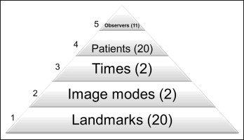
In our study, the multilayer correlations were induced by the following 5 levels of clustering: level 1, 20 cephalometric landmarks in 1 patient (cluster size of 20); level 2, imaging modes of conventional vs CBCT imaging systems (cluster size of 2); level 3, repeated measurements at 2 time points (cluster size of 2); level 4, 20 patients (cluster size of 20); and level 5, 11 observers who conducted the identification procedures (cluster size of 11). Figure 3 shows the hierarchical structure of this 5-level clustered design. Notably, the observations at 20 landmarks were put together, and the measurements from times 1 and 2 were not averaged so that the landmark effect and the potential temporal effect could all be examined simultaneously. To sum up, at each of the 20 landmarks, 880 observations were collected from 2 modes × 2 times × 20 patients × 11 observers (2 × 2 × 20 × 11 = 880), and thus a total of 880 × 20 clustered observations obtained from this 5-level clustered design were analyzed by fitting 1 multiple linear regression model.
In addition to those clustering variables, basic patient information (age, sex, metallic dental restorations, and facial asymmetry), location of the landmark (on the midsagittal plane or bilateral structures), characteristics of the landmark (skeletal or dental), and seniority of the observer (level 1 or 2 for the first or second year in our 3-year graduate orthodontic residency training program) were considered as explanatory variables in the generalized estimating equations analysis. In particular, a new variable, “vision,” was created to classify the 20 landmarks into 3 categories according to their visibility on the cephalograms. Vision 0 was for landmarks on the structures with high image contrast such as S, Gn, and Go; vision 1 was for landmarks on the structures with low image contrast such as N, ANS, A, B, Pog, Me, Ar, and PNS; and vision 2 was for landmarks on the structures with multiple overlapping images such as Or, U1R, L1R, Po, Ba, UMo, and LMo. Although the regression analysis of the clustered data by using the generalized estimating equations model seemed to be complicated, we could comprehensively and simultaneously evaluate the relative impacts of many variables potentially affecting landmark identification errors.
Results
Table II shows the significant variables for landmark identification errors and their regression coefficient estimates in the multiple linear regression model by using the generalized estimating equation method. First, the variable “image modality” was not included in the final model; thus, the differences between the 2 imaging modes (conventional vs CBCT-derived) did not reach statistical significance. However, the landmark identification errors significantly increased at ANS (0.79 mm), A (0.82 mm), L1R (0.44 mm), B (0.60 mm), Me (0.20 mm), Go (0.50 mm), Ba (1.42 mm), PNS (0.68 mm), and LMo (0.19 mm), but decreased at S (−0.37 mm), Or (−0.99 mm), and L1 (−0.12 mm). Only some of them, including ANS, A, B, Go, Ba, and PNS, reached clinical significance (0.5 mm). Having significant interactions with the CBCT imaging mode, the landmarks N (0.35 mm), Or (0.18 mm), and ANS (0.18 mm) exhibited the positive values of the regression coefficient estimates, implying that the identification error increased at N, Or, and ANS on the CBCT-derived cephalograms. In contrast, the negative values of the regression coefficient estimates for Pog (−0.16 mm), Gn (−0.40 mm), Me (−0.37 mm), and Ba (−0.76 mm) had decreased identification errors on the CBCT-derived cephalograms. As to the temporal effect, only 3 variables had significant interaction with time 2, and the regression coefficient estimates were relatively low.
| Covariate | Regression coefficient estimate | 95% Confidence limits | P value | |
|---|---|---|---|---|
| Intercept | 1.05 | 0.89 | 1.21 | <0.0001 |
| S | −0.37 | −0.44 | −0.30 | <0.0001 |
| Or | −0.99 ∗ | −1.12 | −0.88 | <0.0001 |
| ANS | 0.79 ∗ | 0.66 | 0.92 | <0.0001 |
| A | 0.82 ∗ | 0.72 | 0.91 | <0.0001 |
| L1 | −0.12 | −0.17 | −0.06 | <0.0001 |
| L1R | 0.44 | 0.29 | 0.59 | <0.0001 |
| B | 0.60 ∗ | 0.50 | 0.71 | <0.0001 |
| Me | 0.20 | 0.12 | 0.27 | <0.0001 |
| Go | 0.50 ∗ | 0.39 | 0.66 | <0.0001 |
| Ba | 1.42 ∗ | 1.09 | 1.75 | <0.0001 |
| PNS | 0.68 ∗ | 0.59 | 0.78 | <0.0001 |
| LMo | 0.19 | 0.06 | 0.32 | 0.0033 |
| Male | 0.13 | 0.05 | 0.22 | 0.0026 |
| Facial asymmetry | −0.17 | −0.29 | −0.06 | 0.0038 |
| Metallic restoration | 0.12 | 0.04 | 0.21 | 0.0039 |
| Skeletal landmark | 0.17 | 0.08 | 0.26 | 0.0002 |
| Midsagittal plane | −0.27 | −0.35 | −0.18 | <0.0001 |
| Vision 2 | 1.17 ∗ | 1.08 | 1.26 | <0.0001 |
| Observer 3 | −0.26 | −0.33 | −0.19 | <0.0001 |
| Observer 7 | −0.58 ∗ | −0.70 | −0.45 | <0.0001 |
| Seniority 2 | −0.26 | −0.39 | −0.14 | <0.0001 |
| Interaction with CBCT image mode | ||||
| N | 0.35 | 0.22 | 0.47 | <0.0001 |
| Or | 0.18 | 0.02 | 0.34 | 0.0248 |
| ANS | 0.18 | 0.01 | 0.36 | 0.0401 |
| Pog | −0.16 | −0.27 | −0.05 | 0.0062 |
| Gn | −0.40 | −0.55 | −0.25 | <0.0001 |
| Me | −0.37 | −0.49 | −0.26 | <0.0001 |
| Ba | −0.76 ∗ | −1.12 | −0.40 | <0.0001 |
| Age | −0.02 | −0.02 | −0.09 | <0.0001 |
| Facial asymmetry | 0.32 | 0.11 | 0.53 | 0.0029 |
| Skeletal landmark | 0.16 | 0.06 | 0.27 | 0.0027 |
| Midsagittal plane | 0.22 | 0.11 | 0.34 | 0.0001 |
| Interaction with time 2 | ||||
| Midsagittal plane | −0.10 | −0.19 | −0.02 | 0.0151 |
| Vision 0 | 0.23 | 0.12 | 0.33 | <0.0001 |
| Vision 2 | −0.12 | −0.22 | −0.02 | 0.0183 |
Stay updated, free dental videos. Join our Telegram channel
VIDEdental - Online dental courses


