Introduction
In this study, we investigated the impact of defect size and scan voxel size on the accuracy of cone-beam computed tomography (CBCT) diagnoses of simulated condylar defects and assessed the value of orthodontic CBCT images typically scanned at lower settings (0.4-mm voxel size and full-size field of view) in diagnosing condylar erosion defects.
Methods
Cylindrical holes simulating condylar defects with varied diameters (≤2, 2-3, and >3 mm) and depths (≤2 and >2 mm) were created in 22 fresh pig mandibular condyles, with defect number and size per condyle and quadrant randomly determined. With the soft tissues repositioned, 2 CBCT scans (voxel sizes, 0.4 and 0.2 mm) of the pig heads were obtained from an i-CAT unit (Imaging Science International, Hatfield, Pa). Reconstructed CBCT data were analyzed independently by 2 calibrated, blinded raters using Dolphin-3D (Dolphin Imaging and Management Solutions, Chatsworth, Calif) for defect identification and localization and defect diameter and depth measurements, which were compared with physical diagnoses obtained from polyvinyl siloxane impressions.
Results
Identification and localization of simulated defects demonstrated moderate interrater reliability and excellent specificity and sensitivity, except for extremely small defects (both diameter and depth ≤2 mm) viewed with 0.4-mm scans, which had a significantly lower sensitivity (67.3%). Geometric measurements of simulated defects demonstrated good but not excellent interrater reliability and submillimeter inaccuracy for all defects. Receiver operating characteristic analyses demonstrated that the overall accuracy of diagnosing simulated condylar defects based on CBCT geometric measurements was fair and good for the 0.4-mm and 0.2-mm voxel-size scans, respectively. With the prevalence of condylar erosion defects in the patients considered, the positive predictive values of diagnoses based on 0.5-mm size (diameter or depth) cutoff points were near 15% and 50% for asymptomatic and symptomatic temporomandibular joints, respectively; the negative predictive values were near 95% and 90%, respectively.
Conclusions
When using orthodontic CBCT images for diagnosing condylar osseous defects, extremely small (<2 mm) defects can be difficult to detect; caution is also needed for the diagnostic accuracy of positive diagnoses, especially those from asymptomatic temporomandibular joints.
Approximately 6% to 12% of the population in the United States suffers from symptoms of temporomandibular joint (TMJ) disorders, including pain, limited range of motion, joint sounds, or headaches. Although osseous changes of the TMJ have been radiographically observed in 14% to 44% of these patients with 2-dimensional imaging, more accurate diagnosis is critical for understanding the pathophysiology and designing treatment plans for these TMJ disorders. Clinicians typically use panoramic radiographs, cranial projections, and tomograms to radiographically assess the TMJ and its osseous components, but research has shown the limitations of these imaging modalities. TMJ imaging is inherently difficult because of the small nature of its components and the indistinct image that frequently results from superimpositions with the cranial base. Particularly, the commonly used panoramic radiography for orthodontic patients provides a cost-effective gross depiction of the entire TMJ and might be helpful for the identification of significantly altered bony anatomy of the condyle, but it cannot delineate relatively small osseous lesions at the condylar surface.
Cone-beam computed tomography (CBCT) has been used for routine orthodontic diagnosis and treatment planning by some orthodontists. This imaging tool brings practitioners new opportunities and responsibilities for better diagnosis of structures shown in the CBCT images, including the TMJ. Rendering 3-dimensional images with reduced cost and radiation compared with conventional computed tomography, CBCT was suggested in several recent studies to be a promising tool to diagnose osseous conditions of the TMJ. More specifically, Honda et al demonstrated that CBCT can be used to assess osseous abnormalities of the mandibular condyle, and Katakami et al confirmed that CBCT images can accurately depict large erosive changes of the cortical bone of the condyle. Based on the analysis of simulated spherical lesions in dry human mandibular condyles, Marques et al concluded that overall, CBCT is an accurate method for evaluating condylar lesions, with greater difficulty associated with smaller simulated lesions. On the other hand, Librizzi et al recently reported that the diagnostic efficacy for small erosive condylar changes deteriorates with increases of the field of view and the voxel size of the CBCT scans.
A sound radiographic tool for the diagnosis of condylar osseous lesions must be reasonably reliable and accurate, first in a qualitative aspect for the identification and localization of defects, and then in a quantitative aspect for the measurements of defect dimensions. No previous study, however, has systematically examined both aspects. For example, Marques et al only evaluated the qualitative aspect using condylar specimens without overlying soft tissues; this differs from the situation of clinical patients and tends to introduce errors in CBCT diagnosis. It remains to be investigated how accurately one can measure the size of defects from CBCT images, and how one can determine that a suspected defect is a true defect based on quantitative CBCT measurements of the suspected defect. Conceivably, answers to these questions are important for clinical selection of imaging tools, such as CBCT, especially when condylar osseous defects are suspected. More importantly, for orthodontists using CBCT images instead of conventional panoramic and cephalometric films for diagnosis and treatment planning, the images were often obtained at a lower setting (typically 0.4-mm voxel size and full-size field of view) than those used for the diagnosis of pathology. Whether orthodontic CBCT images provide adequate accuracy for diagnosing condylar defects is currently unknown.
The purpose of this study was to address these questions. Specifically, by simulating osseous defects of varied sizes on pig condyles, which were subsequently scanned under common clinical settings and analyzed by blinded raters, we investigated the impact of defect sizes and scan voxel sizes on qualitative (defect identification and localization) and quantitative (defect size measurements) diagnoses. We hypothesized that the sensitivity of qualitative diagnoses and the accuracy of quantitative diagnoses would increase with larger defect sizes and higher CBCT scan resolutions. Then, in a clinically relevant manner, we assessed the value of orthodontic CBCT images in the diagnosis of mandibular condylar erosion defects.
Material and methods
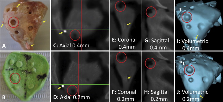
Eleven 3-month-old fresh nonembalmed pig cadaver heads, having a total of 22 condyles (4 quadrants per condyle), were collected from a university animal laboratory immediately after the pigs were killed. Before that, all pigs had received an endoscopic abdominal operation as part of a surgical training program, which was neither a component of nor a disturbance to our study. After making a skin incision around the TMJ area, the subcutaneous soft tissues were dissected to expose the mandibular condyles. The soft-tissue attachments medial to the condyle were then severed; this allowed moving the entire condylar head laterally out of the fossa to be fully exposed. No tissue was removed during these procedures. The articular surface of each mandibular condyle was divided into 4 quadrants (demarcated by grooves with glued gutta percha markers) ( Fig 1 , A ). After excluding 8 quadrants with natural defects (cracks or grooves macroscopically visible on the condylar surface), 80 quadrants were used for defect creation and subsequent analysis. Cylindrical holes simulating condylar defects of 3 diameters (≤2, 2-3, and >3 mm) and 2 depths (≤2 and >2 mm) were created using a dental hand piece and carbide burs (Volvere VMax; Brasseler USA, Savannah, Ga). The mean and range of the actual defect size for each level were obtained from physical measurements of polyvinyl siloxane impressions (detailed below) by 2 raters (A.P. and E.J.). After the defects were created, the condyle was returned to the fossa, and the soft tissue overlying the condyle was repositioned for subsequent CBCT scans.
A prestudy power analysis was conducted based on a hypothesis that the sensitivity of CBCT defect detection would improve from 50% for the smallest defects to 100% for the largest defects; therefore, we determined that a minimum of 16 sites for each defect size was required to reach 90% power. With 2 study sites in each condylar quadrant ( Fig 1 , A ), the number (0, 1, or 2) and the size of the defects were assigned to each quadrant according to a random number table. A negative control site received no defect assignment.
The pig heads were scanned with a CBCT scanner (120 kV, 5 mA i-CAT; Imaging Science International, Hatfield, Pa) using a typical setting for orthodontic records with a field of view (height/width, 10-13/16 cm) and 0.4-mm voxel size (scan time, 8.9 seconds), and a higher (experimental) resolution level of 0.2-mm voxel size (scan time, 26.9 seconds) with the same field of view.
All CBCT data (DICOM files) were subsequently analyzed by 2 calibrated, independent, and blinded raters (A.P. and E.J.) using Dolphin-3D software (Dolphin Imaging and Management Solutions, Chatsworth, Calif) at the same computer monitor setting (1600 × 1200 pixels); they also measured the polyvinyl siloxane impressions detailed below. All DICOM files were randomly coded before analysis to blind the raters to specimen identity. Both raters underwent a training session to learn the software features and a systematic method of viewing the condyles, followed by a calibration session during which they independently analyzed the CBCT scans of 3 randomly selected condyles. The results of qualitative identification and localization and quantitative measurements of the defects were evaluated and compared to ensure that both raters followed the same protocol. More specifically, to analyze each condyle, the raters first oriented the mandibular body to be parallel to the floor in the sagittal view, then oriented the mandibular ramus to be perpendicular to the floor in the coronal view, followed by aligning the medial and lateral gutta percha markers with the line demarcating the coronal slice in the axial view. Using the 4 gutta percha markers, the 4 quadrants were demarcated ( Fig 1 , C and D ).
Then the defects in each quadrant were identified (qualitative diagnosis) primarily in the axial view, supplemented by using the coronal and sagittal views. The 2-dimensional views instead of 3-dimensional volumetric views were chosen because one could check a suspected defect by using multiple consecutive 2-dimensional slices ( Fig 1 , C-H ) but not 3-dimensional volumetric views ( Fig 1 , I-J ). The volumetric views also tended to have artifacts at certain articular surfaces. Subsequently, for every defect identified, its diameter and depth were measured in the coronal (for defects in the anterior quadrants) and axial (for defects in the posterior quadrants) views, which were confirmed to be adequate and consistent during the calibration process. The sagittal view ( Fig 1 , G and H ) was not used for quantitative measurements to prevent redundancy. The diameter was measured at the surface of each defect, and the depth was measured from the condylar surface to the deepest part of the defect. For each identified defect, measurements were obtained from 3 consecutive slices and averaged.
To assess the intrarater reliability of the measurements, the CBCT data of 6 randomly selected condyles were reanalyzed 6 weeks after the initial analysis.
After the CBCT scans, the soft tissues were removed from the pig heads, and the mandibular condyles were separated from the rami using a diamond disk (Brasseler USA, Savannah, Ga), and the intra-articular disc was carefully removed without changing the condylar surface and simulated defects. Light-bodied polyvinyl siloxane impressions were then made of each condyle. The impressions were extended to include the gutta percha markers so that the quadrant designations were also transferred to the impressions ( Fig 1 , B ). After delineating the quadrants and labeling each impression with an indelible marker, 2 calibrated raters (A.P. and E.J.) independently measured the diameter and depth of the positive imprints of the defects using a digital caliper (precision, 0.001 mm) ( Fig 1 , B ). For each defect, each rater measured the depth and diameter in 2 orientations from which the average depth and diameter were calculated. To confirm that the polyvinyl siloxane impression method accurately reflected the actual dimensions of the defects, 6 condyles were randomly selected for both direct and polyvinyl siloxane impression measurements, with 5 months between the 2 sets of measurements.
Statistical analysis
For qualitative diagnoses, the interrater reliability was assessed with kappa tests. The sensitivity and specificity of using CBCT for defect detection and localization were calculated. The change of specificity with CBCT scan resolution levels (0.4 and 0.2 mm) was assessed with McNemar tests, whereas the impact of actual defect sizes and scan resolutions on sensitivity was assessed by chi-square tests.
For quantitative diagnosis, intraclass correlations and Bland-Altman tests were first conducted to assess the interrater reliability of the polyvinyl siloxane measurements, their agreement with the direct physical measurements of the defects, and the intrarater and interrater reliabilities of the CBCT measurements. Then, for all defects that were correctly detected by CBCT, the difference between each set of CBCT measurements and polyvinyl siloxane physical measurements was calculated. The variances between the CBCT and polyvinyl siloxane measurements caused by the factors of scan resolutions, defect dimensions, and the interactions of these 2 factors were tested by 2-way analysis of variance (ANOVA). Bland-Altman analyses of the variability between CBCT and polyvinyl siloxane physical measurements were also performed.
Subsequently, to assess the value of using CBCT quantitative measurements in diagnosing the presence or absence of a true defect, receiver operating characteristic analyses were conducted by plotting the quantitative CBCT measurements against the dichotomized physical truths of defect presence or absence. More specifically, during the diagnosis of CBCT images, the raters first assessed whether and how many defects were suspected in each condylar quadrant and then measured the sizes of the suspected defects. A 0 value was used as the CBCT measurement for a site without a suspected defect. The overall diagnostic values of this method were indicated by the areas under the curves, which were compared between scan resolutions and between actual defect sizes using correlated U statistics. The cutoff point of optimal accuracy (sensitivity and specificity combined) for each voxel size and defect size condition was identified. The sensitivity and specificity values, together with the prevalence ranges of condylar erosion defects reported for human patients, were used to calculate positive and negative predictive values of diagnosing condylar erosion defects by this method.
All statistical analyses were performed with SPSS software (version 19.0; IBM, Chicago, Ill), except for the comparisons between receiver operating characteristic curves, which were run in MedCalc for Windows (version 12.4.0.0; MedCalc Software, Mariakerke, Belgium). An α level of 0.05 was set for all analytical tests.
Results
The physical measurements derived from the polyvinyl siloxane impressions are summarized in Table I . Because these measurements were in excellent agreement with the direct defect measurements and between the raters, the physical measurements from both raters were averaged and used for subsequent comparisons with the CBCT measurements.
| Parameters | Defect size/dimension | Rater 1 | Rater 2 | Average |
|---|---|---|---|---|
| Diameter (mm) | ≤2 | 1.02/2.00/1.48 | 1.01/1.99/1.51 | 1.02/1.99/1.49 |
| >2 but ≤3 | 2.00/2.98/2.46 | 2.01/2.98/2.50 | 2.00/2.99/2.49 | |
| >3 | 3.02/4.31/3.34 | 3.03/4.45/3.37 | 3.02/3.91/3.34 | |
| Depth (mm) | ≤2 | 0.46/1.97/1.09 | 0.35/1.95/1.07 | 0.42/2.00/1.11 |
| >2 | 2.01/2.57/2.17 | 2.01/2.51/2.14 | 2.01/2.45/2.15 | |
| Overall interrater reliability | Diameter | ICC: 0.964; BA: 0.032 ± 0.575 | ||
| Depth | ICC: 0.951; BA: −0.015 ± 0.400 | |||
| Reliability between PVS and direct measurements | Diameter | ICC: 0.999; BA (D direct – PVS ): −0.018 ± 0.113 | ||
| Depth | ND | |||
∗ Correlation coefficient values.
† mean differences of CBCT measurements between the 2 raters.
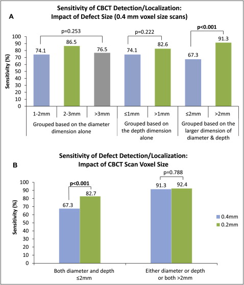
The overall interrater reliability values for defect detection and localization were 0.669 and 0.538 (kappa tests) for the 0.4-mm and 0.2-mm voxel size scans, respectively. The sensitivity and specificity rates of CBCT defect identification ( Table II ) also demonstrated variations between the raters. Overall, the specificity of the CBCT diagnosis had a range of 79.2% to 91.7%, and there was no statistical difference between the 0.2-mm and 0.4-mm voxel size scans for either rater (McNemar test, P = 1.000). The sensitivity of the CBCT diagnoses had a range of 72.9% to 87.5% and tended to increase with a higher (0.2 mm) scan resolution. When the defects were grouped based on either diameter or depth dimension alone, there was no statistical difference of the sensitivity measurements among the groups. However, when they were grouped based on the greater dimension of the diameter or the depth, relatively large defects (at least 1 dimension >2 mm) had significantly higher sensitivity than relatively small defects (both diameter and depth ≤2 mm) ( Fig 2 , A ). With the increase of scan resolution, the sensitivity rates improved significantly for relatively small defects but not for relatively large defects ( Fig 2 , B ).
| Scan voxel size (mm) | Specificity (%) | Sensitivity (%) | |
|---|---|---|---|
| Rater 1 | 0.4 | 83.3 | 80.6 |
| 0.2 | 79.2 | 87.5 | |
| Rater 2 | 0.4 | 91.7 | 72.9 |
| 0.2 | 87.5 | 81.3 | |
| Average | 0.4 | 87.5 | 76.7 |
| 0.2 | 83.3 | 84.4 |
The intrarater and interrater reliability values of the CBCT measurements are shown in Table III . All intrarater reliability measurements, except for 2, were above 0.8, and all interrater reliability measurements were above 0.7. Analyzed by the Bland-Altman method, almost all intrarater and interrater variability values had average errors near 0 and limits of agreement ranges near 1 mm.
| Scan voxel size (mm) | Intrarater reliability (rater 1) | Intrarater reliability (rater 2) | Interrater reliability | |
|---|---|---|---|---|
| Diameter | 0.4 | ICC: 0.92 | ICC: 0.84 | ICC: 0.73 |
| BA: 0.02 ± 0.58 | BA: −0.12 ± 0.76 | BA: 0.08 ± 1.06 | ||
| 0.2 | ICC: 0.80 | ICC: 0.80 | ICC: 0.79 | |
| BA: 0.08 ± 0.97 | BA: −0.01 ± 1.03 | BA: 0.11 ± 0.99 | ||
| Depth | 0.4 | ICC: 0.48 | ICC: 0.81 | ICC: 0.72 |
| BA: 0.07 ± 1.33 | BA: −0.14 ± 0.63 | BA: −0.09 ± 0.78 | ||
| 0.2 | ICC: 0.80 | ICC: 0.64 | ICC: 0.78 | |
| BA: −0.01 ± 0.68 | BA: 0.01 ± 1.10 | BA: −0.10 ± 0.69 |
∗ Correlation coefficient values.
† mean differences of CBCT measurements between the 2 raters.
Two-way ANOVA analysis was used to test whether the actual defect sizes and CBCT scan voxel sizes cause systematic errors to CBCT measurements. The results were similar between the raters; only those from rater 1 are shown in Table IV . When defect diameter was assessed, there was a significant interaction between the actual defect size and the CBCT voxel size factors. More specifically, for defects with a diameter of 2 mm or less, there was a mean overestimation of CBCT measurements for the 0.4-mm scans, but not for the 0.2-mm scans; for defects with a diameter greater than 2 mm, there were nearly identical underestimations for both voxel size scans. Similarly, when defect depth was assessed, we found an overestimation for relatively small defects (physical depth, ≤2 mm) but an underestimation of relatively larger defects (physical depth, >2 mm) ( Table IV ). Overall, all the average CBCT overestimations and underestimations of defect dimensions were less than 0.5 mm.
| Factor | Level | D CBCT-Phy : mean ± SD (mm) | F value | P value | |
|---|---|---|---|---|---|
| Diameter | Voxel size | 0.4 mm | −0.185 ± 0.687 | 4.719 | 0.031 |
| 0.2 mm | −0.280 ± 0.590 | ||||
| Diameter | ≤2 mm | 0.109 ± 0.512 | 52.800 | <0.001 | |
| >2 mm | −0.431 ± 0.622 | ||||
| (Voxel size*diameter) | 0.4 mm∗≤2 mm | 0.298 ± 0.532 | 5.628 | 0.018 | |
| 0.4 mm*>2 mm | −0.439 ± 0.621 | ||||
| 0.2 mm*≤2 mm | −0.049 ± 0.440 | ||||
| 0.2 mm*>2 mm | −0.424 ± 0.627 | ||||
| Depth | Voxel size | 0.4 mm | 0.132 ± 0.446 | 0.035 | 0.825 |
| 0.2 mm | 0.128 ± 0.407 | ||||
| Depth | ≤2 mm | 0.117 ± 0.399 | 21.761 | <0.001 | |
| >2 mm | −0.185 ± 0.471 | ||||
| (Voxel size*depth) | 0.4 mm*≤2 mm | 0.185 ± 0.421 | 0.147 | 0.701 | |
| 0.4 mm*>2 mm | −0.208 ± 0.467 | ||||
| 0.2 mm*≤2 mm | 0.170 ± 0.379 | ||||
| 0.2 mm*>2 mm | −0.163 ± 0.490 |
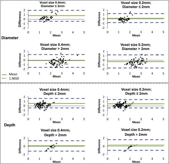
Bland-Altman parameters depict limits of agreement (SD, ±1.96) between the CBCT and the physical measurements, with a larger value indicating greater disagreement. There was general similarity between the 2 raters, and only the results from rater 1 are shown in Figure 3 and Table V . Overall, an individual CBCT measurement of defect diameter is likely to deviate from the physical measurement by 1.05 to 1.35 mm, whereas an individual CBCT measurement of defect depth is likely to deviate from the physical measurement by 0.75 to 1.05 mm. With the defect size factor kept equal, generally, 0.4-mm voxel size scans had a slightly larger limit of agreement than did the 0.2-mm voxel size scans.
| Parameter | Voxel size (mm) | D CBCT-Phy ± Bland-Altman LOA (SD, 1.96) | ||
|---|---|---|---|---|
| Dimension ≤2 mm | Dimension >2 mm | Combined groups | ||
| Diameter | 0.4 | 0.298 ± 1.042 | −0.439 ± 1.218 | −0.185 ± 1.346 |
| 0.2 | −0.050 ± 0.862 | −0.423 ± 1.228 | −0.280 ± 1.155 | |
| Depth | 0.4 | 0.185 ± 0.824 | −0.209 ± 0.918 | 0.132 ± 0.874 |
| 0.2 | 0.170 ± 0.742 | −0.163 ± 0.957 | 0.128 ± 0.797 | |
Stay updated, free dental videos. Join our Telegram channel
VIDEdental - Online dental courses


