In the previous article, we discussed the problem of confounding and presented 3 fundamental methods for assessing and adjusting for confounders: the traditional approach, the noncollapsibility approach, and the directed acyclic graphs (DAGs) or causal diagrams approach.
DAGs are nonparametric structural methods to identify potential confounders through the presentation of variables and the relationship between them in the form of a graph.
A DAG depicts the relationship between the exposure (E) or intervention and the disease (D) or outcome in addition to any other variables associated with E and D.
The first step in building a causal diagram is to determine the effect of E on D independent of all other associated variables or paths. The second step is to statistically assess conditional independence in the causal diagram.
Independence means that our knowledge of 1 variable would not influence our understanding of the other variable. For example, knowing the skeletal maturational age of a patient will not influence our knowledge about the patient’s sex. Thus, skeletal maturational age and sex are independent of each other.
Conditional independence is when we must condition on a third variable to study the relationship between E and D. We condition on a variable by adjusting for it at the design stage (stratification, restriction, or matching) or at the analysis stage (multivariable analysis) of a study. For example, if we studied the effect of orthodontic miniscrew diameter (E) on the initial orthodontic miniscrew stability (D) and found no effect of E on D, then both variables are independent. However, we know from previous studies that initial miniscrew stability is influenced by cortical bone thickness “S,” but miniscrew diameter is not. Thus, we need to condition on cortical bone thickness when assessing the effect of E on D. If we find no association between E and D, then they are independent of each other, conditioning on “S”; hence our knowledge of E will not influence our knowledge of D, conditioning on “S.”
To discover conditional independence in a DAG, we use the concept of directional separation, also known as d-separation. This concept is important in determining whether adjusting for a variable will control confounders or result in bias.
The concept of directional separation
In the preceding article, we defined a path as a sequence of directed edges. A path could be unblocked or blocked depending on certain rules. An unblocked path implies association, and a blocked path implies independence.
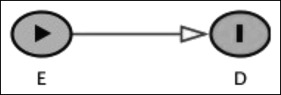
If a path is unblocked (connecting path) between E and D, then there is an association or causation between them ( Fig 1 ). E and D are therefore dependent (d-connected, not d-separated) on one another. This association or causation may not be factual; rather, it can simply be due to bias.
Not all paths convey connecting associations. Some paths are blocked because of the presence of a node that is a collider. We previously defined a collider as a common effect of E and D. It is a variable in which 2 arrowheads converge and appear to collide on the node. We can have different path types in 1 causal diagram.
The concept of d-separation is guided by rules. By applying those rules, one can identify the path’s status (blocked or unblocked) and determine whether adjusting for a variable is needed. This is important to prevent unnecessary adjustment and false associations.
Rules of directional separation
Rule 1. A path is closed or blocked if it has at least 1 collider.
The collider blocks the path between E and D; as a result, the variables become statistically independent of one another (d-separated). A variable could be a collider on 1 path and a noncollider on another in the same causal diagram.
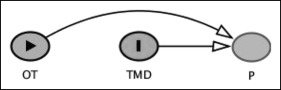
Let us say that we want to investigate the association between orthodontic treatment “OT” (E) and temporomandibular joint disorders “TMD” (D) in a case-control study, with “P” denoting pain; “C” represents patient’s age, which can impact “OT” and “TMD.” We have established that “OT” and “TMD” are statistically independent (relative risk/odds ratio = 1); hence, there is no direct arrow between the 2 variables. Nonetheless, the 2 variables share a common effect, which is “P.” “OT” is associated with “P,” and the same can be said for “TMD.”
In Figure 2 , we can see 2 arrowheads coming from “OT” and “TMD” and colliding into “P.” As a result, “P” becomes a collider, and “P” now blocks the path from “OT” to “TMD”, making the 2 variables independent of each other.
Rule 2. Conditioning on the collider unblocks or opens the path between E and D.
We learned that a collider or a common effect blocks the path between E and D. However, if we adjust for this collider (at the analysis or design stage), we open a supplementary path between E and D that should have stayed blocked. As a result, we induce a false association between E and D (also known as collider bias or endogenous selection bias).
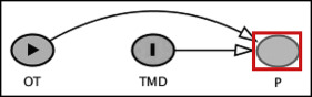
Referring back to our previous example on the association between “OT” and “TMD,” we know that “P” blocked the path between “TMD” and “OT” ( Fig 2 ).
If we condition on “P” (to indicate that a variable has been conditioned on in a DAG diagram, we draw a square box around the conditioned-on variable), we open the path between “OT” and “TMD” through “P” and introduce a spurious association between “OT” and “TMD” that may not truly exist ( Fig 3 ).