Rheology
An important behaviour in nearly the whole of dentistry is that of flow. This subject addresses dynamic aspects of the deformation of materials picking up themes that were introduced in Chapter 1, which was otherwise more to do with static tests. However, no sharp division exists between the two areas. While ‘static’ tests tend to be concerned with the final outcome, flow focuses on deformation while it is happening. Rheological considerations are involved in many types of material, including impression materials, restorative materials and cements, waxes and the casting process. It is also highly important in the context of gypsum product slurries.
Simple analogue mechanical models again provide a useful means of classifying the types of process. By dealing with the model elements in this way, more complicated systems can be dealt with simply in terms of additive effects. These elements are the Hookean spring and static friction block as before, but now adding the Newtonian dashpot.
A simple classification of flow behaviour shows the implications for the handling of real materials. For proper control of mixing, impression taking, model pouring and so on, the flow properties must be taken into account.
An example of detrimental flow behaviour is illustrated by the compression set test, applicable to flexible impression materials which suffer deformation during removal from the mouth. The permanent deformation that results is the major source of dimensional inaccuracy.
Fillers are very widely used to modify the properties of materials, usually by increasing the viscosity of the medium in which they are suspended. However, the amounts that can be used are limited, and this is another source of compromise that must be accommodated in the design of materials.
Some examples of flow systems of importance are discussed, including settling, waxes, and through tubes.
In practically every aspect of dentistry the flow of a material is vitally important to the outcome of the procedure: taking impressions, pouring models, making wax patterns, investing, casting, cementing, fissure sealing and placing restorations are just some of these aspects. Such procedures are essential because only very rarely will the material for a procedure or a device not be required to flow or deform plastically at some stage, and no practical substitute methods for the same purposes can presently even be imagined which do not involve flow at one stage or another. In view of the likelihood that flow processes will remain part of dentistry, some appreciation of these phenomena should be gained.
§1 First Thoughts
Rheology is concerned with the time-dependent deformation of bodies under the influence of applied stresses, both the magnitude and rate, whether the bodies be solid, liquid or gaseous. That is to say, the plastic deformation or flow of the material is the focus. The discussion of the mechanical properties of solids (Chap. 1) centred largely on the stress limits below which elastic behaviour is observed or outright failure does not occur. Nevertheless, plastic deformation was of importance in considering toughness, and it is central to the outcome of an indentation hardness test. However, it is usually considered as an essentially instantaneous response to the stress in those contexts. It was only when we considered creep (1§11) that the rate of deformation as such assumed any importance. Yet it should be clear from the idea of a relaxation time (1§9) being applied to all processes at the atomic or molecular levels, and especially from the time-dependent behaviour of polymers (3§5), that it may be difficult, even dangerous, but certainly misleading, to ignore the rate at which these events occur. Then again, in making the distinction between the assumed instantaneous recovery of elastic deformation and the permanency of plastic deformation in solids, it was as if there were no other kind. In the case of fluid flow, superficially it would seem that only permanent plastic deformation is possible, but a great many solids and liquids exhibit time-dependent recovery of deformation, a kind of slow elasticity, and this behaviour must be included too in a general description of rheology.
‘Description’ here is the important word, for we will not attempt to explain rheological properties in terms of detailed atomic or molecular processes but rather resort only to bulk, macroscopic accounts of the responses to applied stresses, except for broad indications of mechanisms in one or two special cases later. Nor is this necessary. In other words, we can ignore atomic and molecular level structure, and treat the materials as continua. For the time being, this phenomenological approach will be entirely sufficient to understand the terminology, the observations, and the practical implications of the various kinds of behaviour in the applications of the materials exhibiting those properties. Certain structural aspects can then be introduced to provide physical explanations of events where these are relevant to the formulation or handling of a product. In practice, failure to recognize these structural causes may lead to faulty technique and wasted work.
§2 Elasticity
Elasticity is ordinarily thought of as an instantaneous response to an applied stress, and does not appear to be a time-dependent property to our general perception. It was shown, however, that even truly elastic deformation takes time (1§9). However, flow is about permanent deformation, and elasticity is by definition completely reversible. Nevertheless, there are two reasons why it must be included in any discussion of rheology. Firstly, all materials exhibit some elastic behaviour. Even undeniable liquids such as water have a compressibility, that is, a finite bulk elastic modulus (1§2.6) as demonstrated by hydrostatic testing. The conduction of sound (an elastic tension-compression wave) through any medium is a consequence of this. Thus, if we are to attempt a general description of deformation, elasticity is necessarily included. Secondly, it will be shown that the idea of instantaneous pure elasticity is but one extreme of the whole range of possible rheological behaviour, and that it is logically and mathematically part of the overall descriptive equation. We cannot ignore it in this context and it is, therefore, dealt with here.
As before, we draw attention to the fact that the term elasticity only implies a return to zero strain at zero stress, without regard to the linearity of the deformation (1§2), the distinction between Hookean and non-Hookean systems being essentially irrelevant and unnecessary (if we were to be excessively pedantic, no material is Hookean, see 10§3.6). However, to simplify the description we will now only refer to Hookean deformation as the ideal behaviour, although this must be understood to be without prejudice to the possibility of other elastic responses. Furthermore, we must make the same restriction as before (1§2), but now in respect of all processes, that the geometry is unchanged by the deformation – an impossibility except in particular special cases, but a basic working approximation.
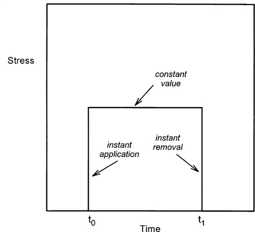
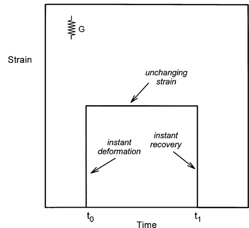
Since now we are interested in behaviour with respect to time, we will plot responses to changes in applied stress and introduce the notion of the stress pulse (Fig. 2.1). That is, a constant stress is to be applied instantaneously to a body for a fixed period of time and then removed completely, again instantaneously. We may then plot the corresponding strain against time (Fig. 2.2). Ideal solids stressed in their elastic region, that is below the yield point if there is one (1§3), always return exactly to their original dimensions upon release of the stress. But, while the constant stress is being applied there is no change in the strain whatsoever. This is obviously implicit in the relevant equation (1§2.5) as time does not appear there as a variable.
The above result applies for any kind of stress, but because flow requires shear, in the present context it will be implicit that shear stress (τ), shear strain (γ), and shear modulus of elasticity (G) are meant exclusively. Unfortunately (for the novice), it is conventional to represent the ideal elastic body by a simple coiled spring loaded in tension for its mechanical analogue (cf. 1§5). It must be remembered that this is only a conventional model representation, and one which has been adopted simply because of the inconvenience of drawing a corresponding shear model.
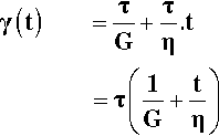
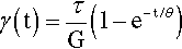
We may then write the shear deformation equation for the Hookean body as follows:
< ?xml:namespace prefix = "mml" ns = "http://www.w3.org/1998/Math/MathML" />

The important addition to this equation is the notation for time, t, at which the observation is made: read “γ(t)” as “shear strain at time t”. This serves as a reminder that the stress which has been applied is explicitly a function of time. Nevertheless, time does not appear on the right hand side of the equation. The units are as before: stress in pascals (Pa), as is the modulus of elasticity, while the shear strain is dimensionless.
§3 Newtonian Flow
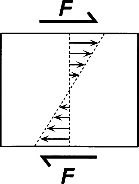
It is basic to the idea of flow that there is shear. No relative movement of one part of a continuous unbroken body with respect to another adjacent part can occur without shear. All descriptions of flow thus depend on shear images. The shearing that occurs in fluids as they flow is perhaps best visualized as between two parallel plates (Fig. 3.1), extending the idea of Fig. 1§2.8. It is a requirement now that the material of the plates is wetted by the fluid so that there is a layer effectively stationary on the surface of each, the boundary layer. In the absence of an applied force, nothing happens. The system is static and at equilibrium.
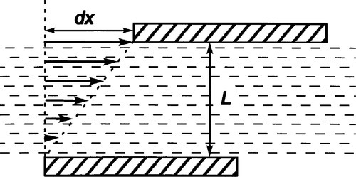
If now a force is applied to the upper plate, acting in its plane (and that of the page in Fig. 3.1), that plate is expected to move with respect to the lower plate (which we will hold stationary for reference). In so doing, the boundary layer to the top plate is carried along, and this in turn tends to cause the next layer to move in the same sense by a frictional effect, and so on from layer to layer to the opposite boundary layer and plate. Thus, the relative motion of one layer exerts a shear force on the next layer. This establishes the shear gradient across the thickness of the fluid. There is complete uniformity across that thickness in the force acting between layers and the relative velocity of one layer with respect to the next. This is the principle of uniformity again.
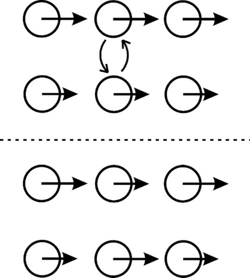
The friction between layers is generated by the transfer of momentum. In a fluid, all molecules have kinetic energy by virtue of their thermal velocities: they diffuse. These velocities have, of course, a wide range of values, but more importantly the directions of travel are random. Thus, in a non-flowing system, some molecules will move from one region to another and other molecules in the opposite direction, on average in equal numbers and on average with identical total momentum (just opposite sign). The net effect is no change. However, in a system undergoing shear, it is clear that one layer is moving faster in the shear direction than an adjacent layer (Fig. 3.2). All molecules in that faster layer thus have a little more momentum in that direction than those in the slower layer. Thus, if some molecules are exchanged between those layers, by diffusion, the net effect is to reduce the total momentum of the faster layer, and to increase it in the slower layer – in the direction of shear. The faster layer therefore suffers friction, slowing it down, whereas the slower layer tends to be speeded up. Ultimately, the momentum is transferred to the moving plates (in a system such as that of Fig. 3.1), and this therefore represents work done by the external system. The same principle applies for polymers, whose macromolecules clearly cannot be exchanged in this way. Instead, the effect is served by chain segments (loops of backbone) and side groups.
The representation of a single force is, of course, a simplification. In fact, there exists across the fluid a turning moment because, by Newton’s Third Law, there must be an equal and opposite force acting on the lower plate when this is stationary (Fig. 3.3). It is conventional to ignore that moment, but its existence should not be forgotten. Now, because any fluid flow, no matter what the geometry, is dependent on shear between adjacent layers, any general remarks applicable to the simple system of parallel plates can be extended to the more complicated systems of actual applications. In fact, all practical rheometers, devices for observing and measuring rheological behaviour, have more complicated geometry because of the practical difficulty of building a machine on the basis of Fig. 3.1. This does not detract from the usefulness of the model.
•3.1 Velocity gradient
Because the material between the plates is a fluid, it therefore responds continuously to the applied shear stress. Thus, in order to maintain that stress across it, and therefore maintain the shear gradient, the upper plate must be kept in motion. It might reasonably be expected that, ignoring accelerations, a constant rate of displacement of the upper plate would require the application of a constant force, when no other aspect of the system is changing. There is now an explicit involvement of time in describing behaviour, since the equation for the displacement in the x-direction of the upper plate in unit time is its velocity v (with respect to the lower plate):
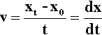
From the definition of shear strain (equation 1§2.20), for the fluid thickness L, the increment of shear strain developed for the increment dx in the displacement of the upper plate is given by:

But this has occurred in increment of time dt, hence the rate of change of shear strain is given by:
The last symbol,  , (say ‘gamma dot’) is a common shorthand for this quantity (the dot means the first differential with respect to time). This shear strain rate is also called velocity gradient, as can be seen from the form of v/L (see Fig. 3.1). Then, following the style of calculation of an elastic deformation (1§2), the shear stress can be related to the shear strain rate by a constant of proportionality, a sort of modulus of flow:

Thus, in our idealized system, for a constant applied shear stress the rate of change of shear strain is constant. On removal of the stress the accumulated strain remains fixed at its last value; there is no recovery of strain because there is no elastic aspect to such a system. That is, there is no driving force to return the system to its original state – no stored energy. We might suspect this because all the work was being done against ‘friction’ between layers, and the energy put in was therefore dissipated, not stored. This was the basis of Joule’s experiments on the mechanical equivalent of heat (c. 1847) in which water was stirred – stirring causes flow, and flow depends on shear. However, the temperature rise must change viscosity, because diffusion is an activated process, and care must be taken experimentally to control temperature. In some circumstances, the heat of mixing will also affect reaction rates.
•3.2 Viscosity
The modulus η is called the coefficient of viscosity of the fluid. It is defined as a constant of proportionality, just as E and G are constants of proportionality in Hookean solids:

Equation 3.4 is Newton’s Law of Viscosity, and a fluid with this type of response (its behaviour) is described as Newtonian, or said to be showing pure flow. The shear deformation equation, that is, the amount of strain produced in a given time at a constant stress, for the Newtonian body is therefore:

Time is now explicitly present on the right hand side. This therefore is time-dependent behaviour. Stress is still in pascals, so the viscosity – the resistance to flow of a fluid – is expressed in pascal-seconds (Pa.s). The important aspect of the system now therefore is that the fluid suffers continuous deformation whilst a stress is applied (Fig. 3.4). Thus, applying the stress pulse of Fig. 2.1 to a Newtonian fluid, the behaviour illustrated in Fig. 3.5 is observed: steadily increasing deformation whilst the stress is applied, no subsequent change when it is removed. The greater the viscosity (i.e. the value of η), the shallower the slope of the plot of strain against time.
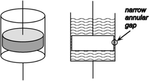
The mechanical analogue for a Newtonian fluid body is the so-called “dashpot”. This is represented as a cylindrical vessel containing a loosely fitting disc or piston immersed in a (Newtonian!) fluid such as oil (Fig. 3.6). When a force is applied to the piston the fluid is forced through the narrow annular gap. Since the gap is small, a small portion of the circumference approximates the appearance of Fig. 3.1, where the upper plate is a portion of the piston and the lower plate the wall of the container. It is this real mechanical equivalent that leads to the use of the model and the symbol. Such devices are in fact used in shock-absorbers for motor vehicles and energy-absorbing buffers of various kinds, “dampers”.
§4 The Maxwell Body
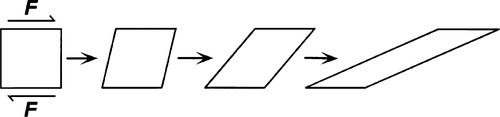
Having developed the ideas of the two extreme forms of deformation, ideal elasticity and ideal flow, we may proceed to consider the intermediate conditions which are more realistic for most real materials. The easiest way to do this is by continuing the model-building approach, using the two ideal mechanical analogues as elements, and examining the behaviour of these models.
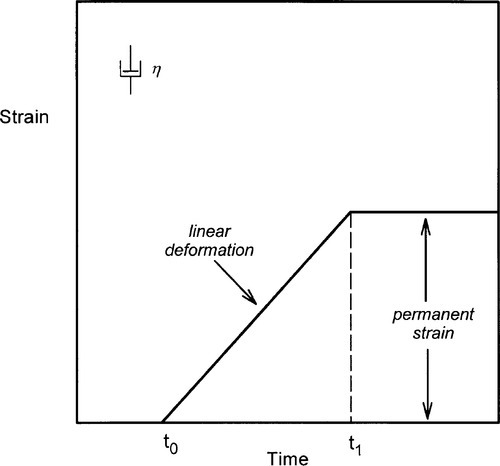
The simplest combination of the spring and dashpot is one of each in series (Fig. 4.1). A material showing the corresponding kind of behaviour is known as a Maxwell body. When the instantaneous stress of the pulse of Fig. 2.1 is applied to this system, the Hookean element responds by extending proportionally to the stress, instantaneously. The deformation due to the viscosity of the dashpot then proceeds linearly with time (since the stress is constant). The removal of the stress at the end of the pulse results in the instantaneous recovery of the elastic strain but, of course, there is no recovery of the viscous strain. The body has therefore suffered a permanent deformation. We can see this directly from the dashpot model – there is no force acting to push the plunger back towards the starting position (there is no energy stored elastically to achieve this). Obviously, any material showing such behaviour could not be expected to retain its original dimensions under any load – even its own weight – for any time. Since there is no yield point (or, equivalently, the yield point is zero), it is in fact little better than the ideal fluid if we want shape retention.
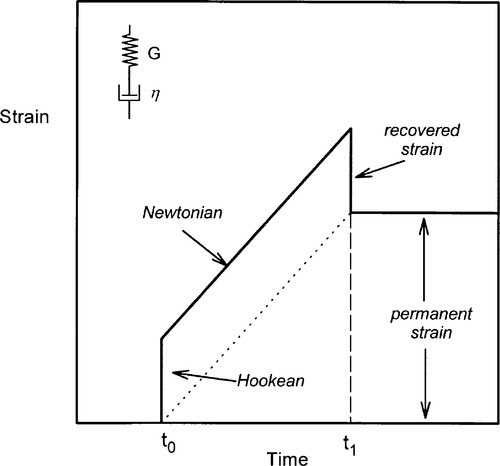
The total strain at any time is the sum of the strains due to the two elements, and the time-dependent and time-independent components are easily written down by combining equations 2.1 and 3.6:
The two strains are therefore algebraically and physically independent of each other, and simply additive. There is no interaction.
On reflection, one can see that such a model must better represent the behaviour of real fluids such as water. We have already noted that water has an elastic modulus (as seen through the existence of its bulk modulus), as indeed must all real liquids. However, the value of that elastic modulus is so high that the deformation produced by the stresses necessary to make water flow is too small to be observed when flow is permitted. Water is therefore a good approximation to a Newtonian fluid because the elastic component in its Maxwell body representation is too stiff to cause any ordinarily noticeable effect. We start to see here how it is the relative magnitude of the two moduli, G and η, that influences the observed behaviour. If η is made large, the graph of Fig. 4.1 approaches that of Fig. 2.2. On the other hand, as G is made large, the graph looks more and more like Fig. 3.5.
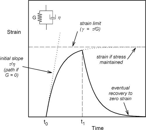
§5 The Kelvin-Voigt Body
The alternative arrangement of the two basic elements, the spring and dashpot, is in parallel (Fig. 5.1). This represents the Kelvin-Voigt body. In this model the extension of the elastic component, the spring, is controlled by the flow in the dashpot. Plainly, no strain can occur instantaneously, since the dashpot requires the elapse of time to move (Fig. 3.5), which is easily seen to be the case even if the value of G were zero. Thus, at t0 the spring is carrying no stress whatsoever. If it were, then it would have extended. There must also be an overall limit to the strain that could occur for a given applied stress if sufficient time were to be allowed. This upper limit will be given by the modulus of elasticity of the spring element exactly as in equation 2.1:
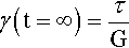
that is, the same result as would be obtained with η = 0. Hence, the stress on the spring alone is zero at t = 0 (since no extension has occurred), and must be τ at t = ∞ (when it is fully extended). Conversely, the stress on the dashpot element is τ at t = 0 and zero at t = ∞. In other words, during the course of the overall fixed stress application, that stress is transferred (in the model) progressively from the dashpot to the spring. Now, the rate of strain depends only on the stress on the viscous element, τv (see equation 3.4), and this stress decreases according to how much strain remains to be accumulated as a proportion of the total strain possible:
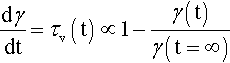
(recall Newton’s Law of Cooling: the rate of loss of temperature is proportional to the temperature excess, 11§2.7). The integration of that differential equation yields the following exponential equation as a result:
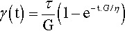
It can be seen that when t = ∞ this reduces to equation 5.1 (e–∞ = 0), and when t = 0

which is one of the defining conditions. It should be apparent from equation 3.6 that this ought to be the case.
The quantity t.G/η, the exponent in equation 5.3, must be a dimensionless quantity (a pure number), and the ratio θ, defined by

can therefore be seen to have the dimension of time (Pa.s/Pa). It is usually known in the rheological field as the retardation time of the system, but it has exactly the same sense as the relaxation time of 1§9; we may use the terms interchangeably to describe the process of approaching equilibrium.
If then we make the substitution in equation 5.3 we get
which shows this idea more clearly. In other contexts, such an exponential term will have a time constant, with units such as s-1, and this would correspond to θ-1, but the sense of the equation remains the same.
•5.1 Reversibility
The important point about the Kelvin-Voigt system is that the entire deformation is recoverable on removing the stress – it is an elastic process. The driving force for this relaxation comes from the stress stored elastically in the spring element – in an ideal system there is no dissipation of energy. It is therefore an internal stress, having no external manifestation except the changes in dimensions.
The rate of strain recovery is controlled by the viscous aspect again, the “dashpot”, and the behaviour of the system can be seen to be entirely symmetrical. The same retardation time (or time constant) applies to this reverse process, and the graph for recovery has exactly the same shape (just inverted) as that for the original deformation. As time is required for the approach to the equilibrium position, whether on initial stressing or during recovery to zero strain, the dimensional changes are said to be damped or retarded. A material exhibiting such behaviour would have to be allowed a certain period to recover after exposing it to any stress if the original dimensions were important, and this will assume considerable significance in the context of impression materials and waxes in particular.
In a sense, Kelvin-Voigt deformation might be thought not to be relevant to flow as such, simply because it is an elastic, recoverable deformation. However, if we take the microscopic view that the movement of an entity from one location to another is what we are concerned about, that process is indeed flow. In any case, if it is only ‘real’ flow that we are concerned about, we still need to be able to identify other components of deformation, as observed in practice, in order to discount them.
In that light, we can see that the Kelvin-Voigt model must be a better representation of the behaviour of real solids in the sense discussed in 1§9. That is to say, if we attempt to measure the elastic modulus of a body by applying a stress, it requires a finite time for the deformation (which we need to measure to calculate the strain) to go to completion. For many solids, that time is so short – of the order of 1 ~ 100 μs (Fig. 1§9.1) – that ordinarily we do not notice the effect. However, when we deal with polymers, where the controlling factor is the movement of chain segments, the relevant time-scale may be far longer (1 ~ 1000 s, or more). Thus, there is no real or clear distinction to be made between so-called static mechanical tests and the rheology of Kelvin-Voigt bodies; it is a matter of the relevant observational time-scale that determines our view of the processes involved. Thus, there can be no such thing as a perfectly Hookean body as in Fig. 2.2 because the response cannot be instantaneous, even though for many purposes it is entirely satisfactory to assume that it is a good working description of actual behaviour.
§6 Viscoelasticity
Many materials, no less in dentistry, show more complicated behaviour than those so far described. We may continue the model-building to consider a series combination of the Maxwell and the Kelvin-Voigt systems (Fig. 6.1). Here we have a combination of an instantaneous elastic deformation, a time-dependent reversible deformation, and irreversible flow, all superimposed. This class of behaviour is called viscoelastic (also known as the Burgers model), and the plot of strain against time for the application of the pulsed stress of Fig. 2.1 clearly shows all of these components.
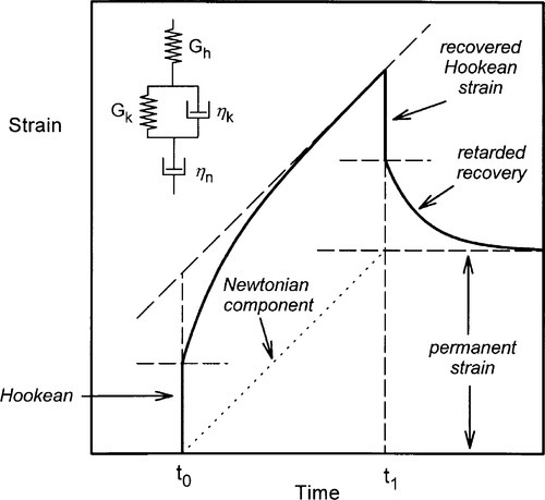
The instantaneous elastic deformation is followed by a stage of decreasing rate of strain as the Kelvin-Voigt component is extended. The Newtonian or pure viscous deformation continues for as long as the stress is applied. On removal of this stress, the Hookean elastic strain is instantaneously recovered, followed by the negative exponential recovery of the Kelvin-Voigt strain. Of course, the Newtonian deformation cannot be recovered, and this is the cause of the permanent strain.
Again, the total strain at any time after the application of the stress can be calculated as simply the sum of the strains from the various components. That is, the system remains purely additive in terms of its individual components. We may write this out algebraically:
where now it is necessary to distinguish between the shear moduli of the Hookean and Kelvin-Voigt components by appropriate subscripts, since they clearly can take different values. Also, θ here is given by θ = ηk/Gk, following equation 5.5, for the Kelvin-Voigt component. Notice, too, that the order of the elements in the model is of no concern, as the sum of equation 6.1 is unaffected by the order of the terms – in other words, both may commute.
If we continue the argument at the end of each of the previous two sections, that is, that the Maxwell body is a better approximation to the behaviour of real liquids and the Kelvin-Voigt body the same in respect of real solids, we can see that the viscoelastic body is a generalization that can accommodate both extremes. The comments about the relative magnitudes of the moduli and the time-scale of observation still apply, as these determine which aspect of behaviour is dominant.
•6.1 Impression materials
This kind of mixed behaviour is shown in a very obvious fashion by all set polymeric dental impression materials, albeit to varyious degrees. Thus, the pure (Hookean) elasticity is a basic requirement if the mould is to approximate the dimensions of the original faithfully; the fact that they are polymers means that the retarded elasticity is noticeable; and various reactions ensure that creep or viscous flow causes enough permanent deformation to reduce the accuracy enough to be important. It can be inferred from this that, so long as applied stresses are of short duration, the purely viscous deformation will be small. But, equally, some little time is required for the full recovery of the reversible strain and the attainment of the maximum accuracy after removal. Hence the recommendation must be for the removal of flexible impressions from the mouth in a single ‘snap’ action (to minimize irrecoverable flow) and for a small delay before pouring the model (to allow for recovery of the retarded deformation – the delay varies between types of material).
It should therefore be apparent that the most important problematic aspect of an impression material is the non-recoverable, viscous deformation, as it is this that ultimately limits the dimensi/>
Stay updated, free dental videos. Join our Telegram channel
VIDEdental - Online dental courses


