Mechanics
Much of the discussion so far has centred on the properties of materials as materials, but even more important is the application of those materials in real objects. It is the behaviour of those objects as engineering structures that is the ultimate goal of those studies. This chapter contains an outline of the mechanical behaviour, essentially the force–deflection characteristics, of some simple structures as encountered in dental applications. This is focused primarily on orthodontic contexts, but is generally applicable to a wide variety of other areas.
A number of foundation concepts are discussed, such as work and moment, and the means of mapping shear stresses and bending moments in a small group of elementary examples. An outline is then given of the principles underlying the development of the equations to describe behaviour, with some examples which may be applied to simple cases.
These ideas lead to the use of flexural rigidity as a descriptor for the behaviour of a beam as an object, combining the effects of material and shape. This is an important element of the design of structures.
A case study is then presented of the application of the above ideas to an orthodontic example, to illustrate the application of the principles and the information that may be deduced concerning the means of modifying designs for specific purposes.
Materials science in dentistry is not to be viewed in isolation. It is its application to real dental products and systems as a means to understand their behaviour that is important. In the case of mechanics it is the engineering principles which control the design and function of devices. This is true whether we are dealing with an orthodontic appliance, a bridge, a denture or an amalgam restoration, or even dental hand instruments.
Dental treatment involves a great variety of different kinds of activity, ranging from the relatively minor interventions of topical medicaments to the complex engineering of orthodontic appliances, although these latter are rarely presented from that point of view. In fact, engineering principles are important in the design of many kinds of dental device: from small fixed bridges, through removable partial dentures, full dentures, the design of impression trays, MOD inlays and direct restorations, to crown posts and beyond. It is at this level that the mechanical properties of materials are put to use, not as tabulated numbers but in the active design process, ensuring that the device will survive and function as intended by choosing the correct dimensions, shape, cross-section, and so on. The purpose of the present chapter is to allow some insight into the behaviour of structures through examples of direct application in orthodontics. The treatment is unavoidably mathematical, but it is largely restricted to algebraic manipulation and all steps are laid out for clarity. Even so, it is the principles of the approach that are of concern, rather than the detail.
In orthodontics various kinds of tooth movement are desired, from bodily displacement (translation) to rotation, in any or all planes, and about any axis. These movements are obtained from the forces applied through stored elastic energy in devices of various types, all of which rely upon a spring in one form or another; the work done in deforming the spring elastically (which is termed ‘activation’ in this area) is recovered as work done on the tooth and supporting structures. Of course, the movements are the result of the active biological remodelling of those supporting structures and not of the simple passage of the tooth through a viscous medium. The speed of response, therefore, is beyond the scope of materials science as such, although the stresses involved in eliciting the physiological response are addressable. In particular, we shall only be concerned with static systems, i.e. at equilibrium, assuming that any motions are so slow as to be safely ignored.
§1 Work and Moment
The basic equation which defines Young’s Modulus, E, for a body under uniaxial stress, σ, was given at equation 1§2.4 a as:
< ?xml:namespace prefix = "mml" ns = "http://www.w3.org/1998/Math/MathML" />

where ε is the axial strain. This equation was obtained to be deliberately independent of the geometry of the system being tested in order to examine material properties in the intensive sense. But in order to study the deformation of real bodies, that is, not in any abstract sense but rather in engineering terms applied to whole structures, we are obliged to consider dimensions. So we retrace our steps slightly. Thus, if the length, L, and cross-section, A, of the test piece are put back, we obtain for the force:
where ΔL is the change in length. Recalling that work done, W (J ≡ N.m), is given by the product of force and the distance, s, moved through, we have:

As the behaviour is assumed to be elastic and linear (i.e. Hookean) the average force (or, equally, the average distance moved) is given by dividing the sum of the extreme values by two. Thus:
This result for the whole object parallels that obtained for the material property of resilience (1§4). This type of analysis is applicable to simple springs of regular shape in compression, tension, shear or bending, irrespective of the form and material, with the sole condition that the device remains Hookean in its deformation characteristics over the range of interest. (If it were not, a more complicated calculation would be required, i.e. of the area under a force-deflection curve – but the principle remains the same.)
In dealing with the sideways deflection of spring elements the idea of torque or (turning) moment, M, has to be introduced. Moment, the tendency of a force to rotate the body to which it is applied, is defined as the product of the force applied and the perpendicular distance d of its line of action to the axis of rotation (Fig. 1.1):

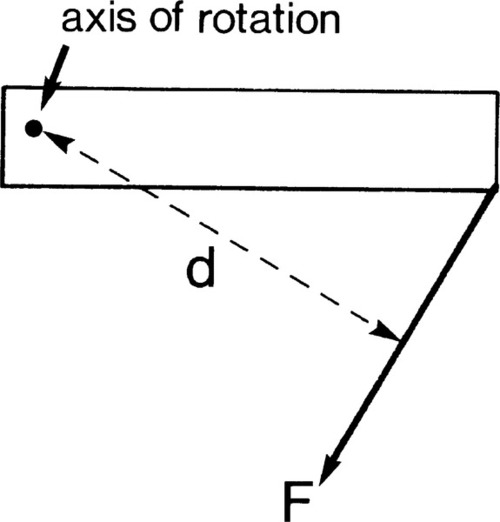
This is seen to be similar to the definition of work, indeed it has the same dimensions – although always expressed as “newton-metres” or some equivalent, but the difference must be carefully noted. In fact, this similarity can be understood in the following sense: for the force to exist in static equilibrium there must be elastic strain in the system, thus work will have been done in reaching the final condition from an initial state of F = 0.
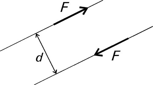
The above definition of moment, however, seems to require that the axis of rotation be defined. This is not strictly necessary. If instead we consider a pair of equal but opposite forces acting along parallel directions, separated by the distance d (Fig. 1.2), then for any point in the plane containing those forces the net moment is a constant, given by equation 1.5, taking into account the sign of the rotation about that point. Such a pair of forces together are said to constitute a moment couple or, simply, a couple.
•1.1 Sign conventions
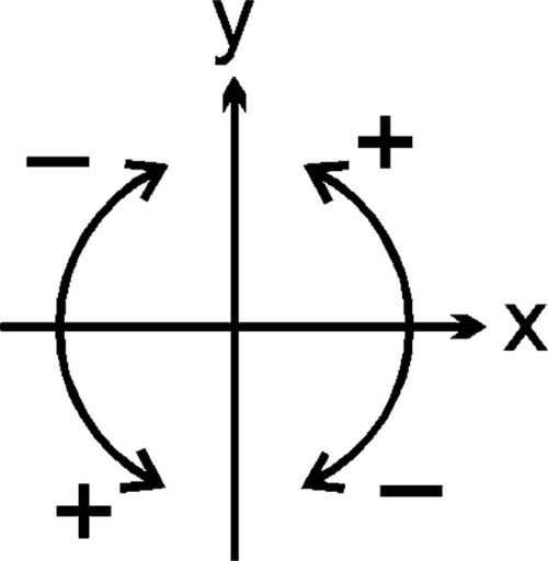
To reach that result we had to establish the sense of rotation. Conventionally, now, anticlockwise rotation is defined as positive and clockwise as negative; the angles moved through in these directions have the corresponding signs (Fig. 1.3). This is the same sign convention as is used for the ordinary definitions of trigonometry.
Note that Newton’s Third Law of Motion says that to any force there is an equal and opposite (in sign or direction) force, i.e. Action = Reaction. Thus, for any moment to exist in an equilibrium system there must be a counteracting moment to establish that equilibrium.
A sign convention also applies to forces, and is implicit in diagrams such as Fig. 1§12.1. Usually, forces acting upwards (+ y direction) are given a positive sign, downwards are negative. Likewise, tension is considered positive while compression is negative.
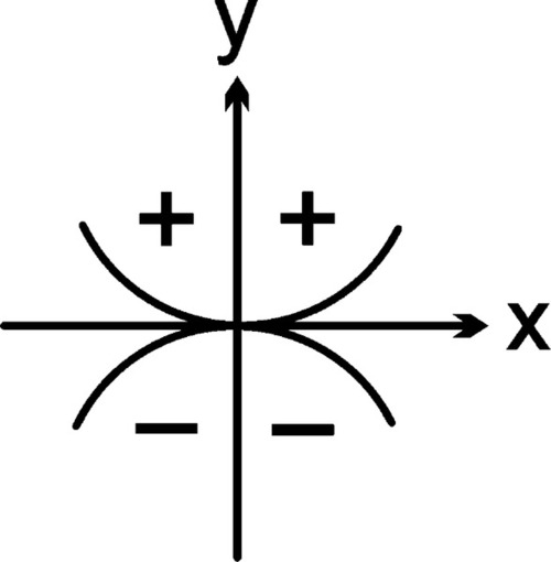
It is also necessary to introduce a convention for the sign of the curvature produced in a bent object. Simply, this takes the sign of the radius of curvature (or, equivalently, the position of the centre of curvature) as indicated by the y-axis, taking the fixed point as the origin (Fig. 1.4). Concave upwards is taken as positive curvature, concave downwards as negative. By quadrant, these are the signs of the sine function. Effectively, since curvature arises from an applied moment (F × d), we need to multiply the sign of the resultant rotation by the sign of the (initial) distance from the origin in the x-axis to get the sign of the moment and thus the sign of the curvature. Notice that the sign of the curvature is unaffected by the choice of origin for the curved element, which is only reasonable.
§2 Simple Beams
Orthodontic appliances, dentures and denture frameworks are complicated structures involving many parts, many cross-sections, and many points of contact with the dentition (and perhaps soft tissues). To understand the way in which they function, and therefore their design, we must begin by considering far simpler systems based on beams, or bars of uniform cross-section, and of material which is homogeneous and isotropic.
•2.1 Cantilever beam
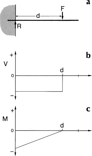
The simplest system is a cantilever beam, one that is considered to be ‘built in’ to the support at one end and so cannot rotate there when the free end is loaded (Fig. 2.1a).[1] The application of a force to some arbitrary point on the upper surface of the beam results in a clockwise moment at the support as before:

But for equilibrium this moment must be opposed by an equal and opposite moment:

This necessary condition is expressed by the equation of moments:

Similarly, the load F must be balanced by a reaction in the support of the same magnitude, but opposite direction:

This similarly essential condition is expressed by the equation of statics:

These named equations of mechanics are alternative versions of Newton’s Third Law. The point is that if equilibrium did not exist the unbalanced forces or moments would cause an adjustment of the geometry, a movement that would establish that equilibrium.
The application of the force F perpendicular to the axis of the uniform section beam means that it is in the plane of a cross-section. It generates a shear between that plane and the adjacent plane of atoms (working in the direction of the support). This is the situation discussed in 1§2 (Fig. 1§2.10). The shear force is transmitted undiminished to the next plane, and so on, all the way to the support. Shear force is constant over the entire length between the point of application of the load and the support (Fig. 2.1b). In addition, for constant cross-section, the shear stress is similarly constant. We give this force a negative sign because it is acting downwards:

It is emphasized that there is no shear stress operating between the point of application of the load and the free end. Because that end is free to move there is by definition no opposition to the deflection, therefore no reaction force, thus no shear.
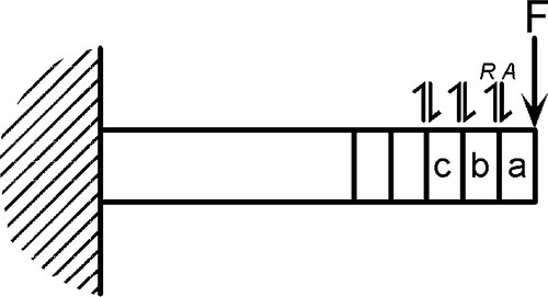
It is worth ensuring that the implications of this are understood. Thus, in Fig. 2.2, the force F creates a shear action A at the interface between blocks a and b. However, since this a system in static equilibrium, there is necessarily a reaction R equal in magnitude to, but opposing A at the same plane. This means that the full force of F is transmitted through block b to the interface between b and c, where a similar argument applies, and so on through the whole beam to the support. By the principle of uniformity (1§2.1) this must be true for all infinitesimal slices of the beam. Thus the shear stress in a uniform cross-section beam is everywhere the same.
The bending moment given at equation 2.1 was specifically calculated as at the support. However, we may also calculate the moment at any point in the beam due to the same applied force. Thus, measuring from the point of application of the load, the bending moment increases as the distance increases:
where x can vary from 0 to d (the reason for writing this in integral form will become apparent below). In other words, within the beam the moment is not constant from point to point but varies directly in proportion to the distance over which it is acting (Fig. 2.1c). Note that the starting point for this integration, the zero distance, is at the point of load application. We have used the force V because we have assigned a sign to this: negative. Thus the moment is also negative. The mechanical interpretation of this is that the centre of curvature is below the beam. Given that the moment can be represented as an integration of the shear force, in the other sense we also have

•2.2 Additivity
Since the purpose of this type of analysis is to be able to handle real systems, as opposed to observing material properties in deliberately simplified mechanical tests (Chap. 1), we now proceed to the case of more than one load applied to the beam. Now, in working with Hooke’s Law (1§2) it is implicit that each increment of load behaves as does any other increment, so that the responses of the system are likewise consistent: we would not have proportionality otherwise. Thus, in Fig. 2.1, it is of no consequence that F is applied as several small loads or as one: the shear force acting at a point is the sum of the shear forces generated by each small load. The response to each load is independent of the responses to other loads (assuming constancy of geometry).
Irrespective of the distribution of the loads on a beam, the total shear force at any point is simply the sum of the shear forces due to all sources:

Thus, for the situation of Fig. 2.3a, the shear force due to F1 operates over the entire distance from its point of application, d to the support, and similarly for F2. Thus, between d and the support both shear forces are acting, but between d and e only the shear force due to F2 is present, since this region is ‘outside’ d. From e to the end of the beam there is no shear. This argument applies equally to bending moments, so that at any point we may write:
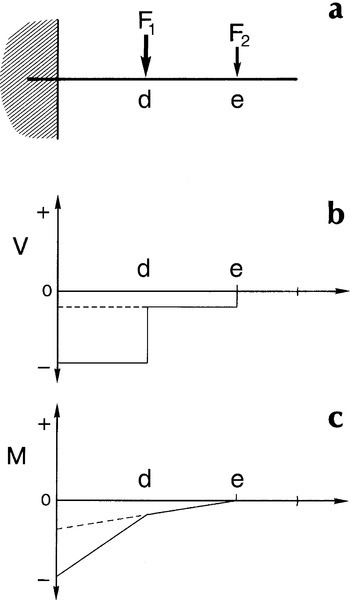
We thus obtain the diagrams of Figs 2.3b and 2.3c by the simple addition of the respective diagrams, in the form of Figs 2.1b and 2.1c, for each of the two forces applied. In fact, if we also assume that the beam is of one uniform material, i.e. constancy of elastic modulus, deflections are also additive:

This simple additivity of the different types of response to the applied loads is called the principle of superposition. That is, assuming constancy of geometry (including magnitudes and directions of the forces applied), the full description of a system can be found as the summation of the effects of each element of load. This is in effect a version of the principle of uniformity (1§2).
•2.3 Self-weight
We can explore the implications of the principle of superposition with a real example. So far the beam has been treated as having no weight, i.e. ignoring the forces felt by the beam due to gravity. The effect of this so-called self–weight of the beam is that of a uniformly distributed load (Fig. 2.4a). Therefore, for a constant weight per unit length of the beam, the load intensity, q, at any point is given by:

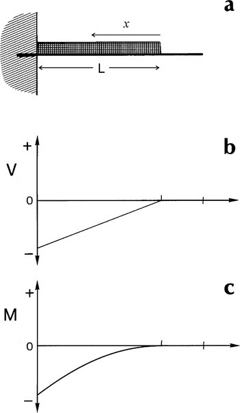
so that the shear stress at a given point depends on the total weight ‘outside’ that point:
Thus, taking the integration route of equation 2.7, we have simply:
where x is measured from the free end. This produces the conditions shown in the diagrams of Figs 2.4 b and 2.4 c. Again, if point loads were to be applied to such a beam, as in Figs 2.1 a or 2.3 a, the separate effects of self-weight and imposed loads can be superposed to find the net effect. The point is that complicated systems can be dissected into their elements to perform the analysis in stages, and the individual results assembled to give the overall picture.
The cantilever is only one form of beam. Another common type is that of the simply supported beam; that is, both ends rest on some (frictionless) support. By the arguments given for the cantilever, the portions outside of the supports (assuming that no forces are applied there) have no influence on the results and will be ignored.
•2.4 Three-point bending
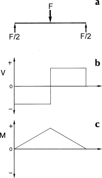
Consider first the situation in Fig. 2.5a. A centrally placed load generates reactions in the supports, each of which is one half of the applied load. This is known as three-point loading and is a common type of mechanical testing arrangement (see Fig. 1§1.3; 1§6.4). Now, looking first at the beam to the left of the central load point, the shear force is acting so as to rotate each element of the beam here clockwise from its original position with respect to the left-hand point of support adopted here as origin. The shear force is therefore negative in sign in this region. Between the centre and the right hand end, however, the shear is acting in the opposite sense, tending to rotate each element of the beam anticlockwise about the centre point and thus must also be acting in the same sense about the adopted origin. The shear force here is therefore positive. The pattern of shear forces is thus as in Fig. 2.5b.
We may dissect the system a little further to clarify this outcome. If we were to take away the right hand support, and thus its reaction, the load to be considered is just F. We then have precisely the load system of a cantilever beam as in Fig. 2.1, with no load, and therefore no shear, to the right of the centre point. On the other hand, if we were to take away the left hand support, and move our reference coordinate system origin to the right hand support, it is a cantilever beam again, with a similar unloaded portion to the left of the centre point, but with the shear in the opposite sense between the centre and the right hand support. We then add the two diagrams together to determine the net effect. It is therefore necessary to observe carefully the sign convention which has been adopted for a consistent picture to be obtained. It is not just a case of identifying ‘up’ and ‘down’, but the sense of rotation as well. This also means that it does not actually matter where we identify the origin of our coordinate system to make such an analysis: the outcome will always be the same.
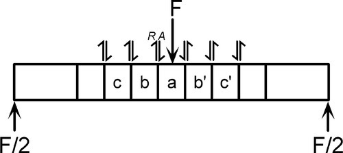
By reasoning similar to that applied for the cantilever beam (§2.1), the shear acting between successive sections of a beam in three-point bending can be shown to be uniform in magnitude (Fig. 2.6). From this it is very clear that the sense of shear changes at the mid-point. If the blocks are imagined to slide, the clockwise motion of a with respect to b, of b with respect to c, and so on, is plain. Similarly, a moves in an anticlockwise sense with respect to b’, and so on. It is the need to distinguish between such conditions that requires the consistent use of a sign convention (§1.1).
Now, to get the bending moment, we apply the integration of equation 2.7 to the shear forces mapped in Fig. 2.5b, from the right and towards our chosen origin at the left hand support. This gives the result shown in Fig. 2.5c. It looks odd at first sight because the moment is everywhere positive, in contrast to the situation in the cantilever beam. However, it is correct because the centre point of the beam must be depressed so that its centre of curvature lies above it, i.e. the curvature is positive, the bending is in the sense of an anticlockwise turn about the origin for all points along the beam. (We would, in fact, achieve the identical result if we chose the right hand support for the origin, because the distance to be used in the integration would then be negative.) We can therefore see that the curvature is the consequence of the imposed system of loads, the outcome and not the causation.
Thus, the overall result for a three-point beam is a shear stress which is uniform in magnitude everywhere except exactly at the centre point (where it is zero), and maximum bending moment, Mmax = FL/4 (i.e. force × distance), at that centre point. Now, if we were doing a mechanical test, if failure occurred it would be due to a flaw initiating the crack. Such flaws would ordinarily be distributed randomly over the test zone, and have a random distribution of size and orientation, so there would be no guarantee that failure would occur at any particular location. This means that the details of the loading at the failure site would vary from test to test because the bending moment varies. However, a slight modification allows a clearer picture to be obtained for some purposes. This involves separating the centre load into two equal portions, symmetrically placed about the centre, to give what is termed the four-point loaded beam (1§6.4).
•2.5 Four-point bending
In a four-point beam the reaction forces are necessarily identical to those in the three-point system (Fig. 2.7a). Following through the same kind of analysis, the shear forces are now found to be restricted to those regions at the ends of the beam between the load application points and the corresponding support, wherein the reaction is seen (Fig. 2.7b). However, considering the force acting on a (Fig 2.8), while it is transmitted to the left and ultimately to the support, it is similarly transmitted to the right to the interface with the central block. But this block is also subject to an identical force – in both magnitude and direction – on the right at the interface with a’. Hence, although being pushed down, the forces acting on the central block are exactly balanced, therefore there is no shear whatsoever.
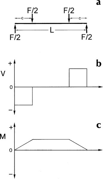
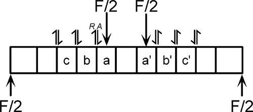
The striking thing here is then the central region in which there is no shear force acting. Notice that, in the limit, if the two upper forces F were moved out to act directly on the supports there could be no shear between the supports, and equally, in the three-point situation (Fig. 2.5a), there is no shear under the coincident pair of forces, each F/2.
The integration for the bending moment is as above, and yields the result of Fig. 2.7c: between the load points it is constant, Mmax = Fc/2, corresponding precisely to the zone of no shear. This region experiences what is therefore known as pure bending.
These examples of beam bending are clearly special cases, being symmetrical, although convenient for mechanical testing (1§6.4), but are illustrative of the main features of and the approach to be taken for more general systems. But shear force and bending moment are not the only effects operating. We must determine what other stresses and strains may be present. For example, it is evident that for any body to be bent, meaning that one surface is made convex and the other concave, the outer convex surface must be relatively longer than a corresponding portion of the inner surface.
Imagine bending a beam into a full circle such that the ends were butted together: the outer surface has a larger radius of curvature; it is therefore longer than the inner surface. Whether this is due to the one being stretched or the other compressed is immaterial. For a relative change in length (i.e. strain) there must be a force acting, and the shear forces identified cannot be the source since shear alone does not change dimensions in that sense. We shall therefore stay with the case of pure bending to investigate this. For either stretching or compression (or both) of those surfaces of the beam to occur means that there are forces acting along its length, perpendicular to the cross-section. Thus, to determine the internal forces operating over any arbitrary cross-section of the central portion of Fig. 2.7a, the deformation of the beam must first be considered.
•2.6 Geometry of bending
For a rectangular beam it is found experimentally that two adjacent parallel lines, mn and pq, on its sides, perpendicular to the length of the beam, remain straight during bending; but also that they rotate (about an axis perpendicular to the page) and remain everywhere perpendicular to the longitudinal ‘fibres’ of the beam (Fig. 2.9a). The theory of bending then assumes this to be a universal result and also, by extension, that the entire section perpendicular to the bending axis remains plane and that every fibre remains perpendicular to that plane. It follows that transverse sections such as correspond to mn and pq (Fig. 2.9a) must rotate as a whole with respect to each other during bending, so that they are no longer parallel.
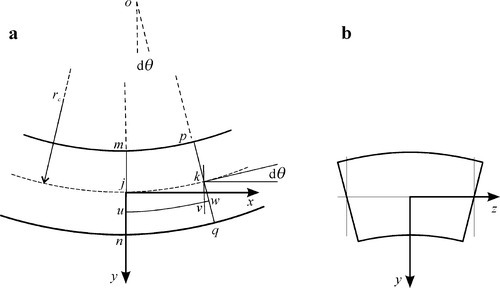
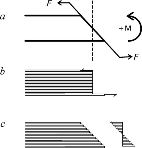
This result can be seen to be expected from an alternative view. Since there is only a bending moment acting on any section of the beam (in the pure bending region), we can represent it as in Fig. 2.10a which shows that, relatively speaking, the upper surface is under compression and the lower under tension, but the magnitudes are as yet unknown. Let us then consider just the extreme outmost fibres (Fig. 2.10b): if the elastic modulus is symmetrical about zero (as is reasonable for small deflections), the deflection of the top fibre must be identical to that of the bottom fibre – but opposite in sign. This means that the net length of the two fibres is unchanged, and that there is therefore no net force acting to extend or compress the pair – which are required conditions for pure bending. The couple is therefore acting to rotate the plane containing the ends of the two fibres about a point midway between the two.
Stay updated, free dental videos. Join our Telegram channel
VIDEdental - Online dental courses


