In the previous article, I introduced the concepts of correlation and regression. In the next articles, I will discuss how we can apply linear regression in orthodontic research with an example.
Research question: We will investigate the effect of the amount of pretreatment crowding (irprtx) on the number of days required to reach alignment (daystoalign). The days to alignment is a continuous variable expressed in days, and the irregularity index is also a continuous variable expressed in millimeters. The assumption is that the greater the initial crowding, the longer it will take to align the dentition.
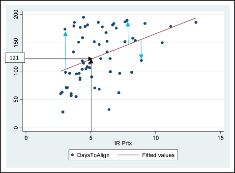
In Figure 1 we can see a linear association between the dependent variable (daystoalign) and the independent variable (irprtx).
The next step is to use this association to predict the number of days required to reach alignment, taking into account the amount of pretreatment crowding. We will use linear regression analysis. This analysis allows us to investigate how much of the variation in the variable daystoalign can be explained by the variable irprtx. The variable irprtx is called the explanatory or independent variable, and the variable daystoalign is called the response or the dependent variable. The goal is to fit a straight line (fitted line or prediction line) to the data that best describe the relationship between daystoalign and irprtx as shown in Figure 1 .
To fit this line, we need to predict the values of the dependent variable for each value of the independent variable using the following equation:
where ∧Yi
Y i ∧
is the predicted i -th value of the dependent variable (daystoalign), X i is the i -th value of the independent variable (irptrx), and α in the intercept, and it determines the point on the y-axis that the fitted line will cross. β is the regression coefficient, and it expresses the amount of change (increase or decrease) in the dependent variable when the independent variable increases by 1 unit. This equation depicts the linear relationship of these variables.
The standard method to fit the regression line is known as least squares regression. This method is based on the vertical distances of the data points from the prediction line that is drawn in a way that minimizes the sum of the squared residuals e (= the distance of the observed data points to the fitted regression line measured on lines vertical to the x-axis: ie, Yi−∧Yi
Y i − Y i ∧
). Each vertical distance is the difference between the value observed for the dependent variable Y and the value of the fitted line ∧Y
Y ∧
for the corresponding value on the x-axis. This vertical distance between the observed and fitted values is known as a residual (e).
The 2 key characteristics of the fitted line are the intercept and the slope. The intercept is the point where the fitted line is expected to cross the y-axis when the value of x is 0. The intercept often does not have a meaningful interpretation; however, it is required to draw the line. The slope corresponds to the coefficient in the regression output, and it indicates the steepness of the line; in other words, this means how much the daystoalign changes for every unit increase of irprtx. A steeper line results in a larger coefficient compared with a less steep line.
In the Table , the regression analysis for the question of interest is shown with the explanation of the table.


