3
Diagnostic Imaging
X- rays were discovered by Wilhelm Rö ntgen in November 1895.1 He was working with a Crookes tube and noticed that when the tube was activated, barium platinocyanide plates lying close by fluoresced. Since he could not see what was being emitted from the tube, he named them X- rays (X meaning “unknown”). Within a few weeks, radiographs of the teeth were being taken independently in Germany, the United States, and England. At this time, dental exposures lasted several minutes and used glass photographic plates wrapped in black paper.
Since then, there have been major developments in equipment design to improve both safety and image quality. Current United Kingdom recommendations for intraoral equipment include the use of highkilovoltage constant potential machines with long focus-to- skin distances and rectangular collimation.2 Film holders and beam- aiming devices are also essential for periapical and bitewing radiography.
Panoramic radiography using a rotating extraoral source of radiation was first patented by A.F. Zulauf in 1922.3 In 1933, a machine using a narrow collimated beam was designed,4 but it is generally accepted that the first rotating panoramic machine was produced by Paatero in Finland.5 The early devices used a single centre of rotation,6 but today’ s modern machines use a continuously moving centre of rotation. This produces a horseshoe- shaped focal layer that corresponds to the shape of the “average” jaws. Accurate patient positioning is important to reduce distortion in the image.
The lateral cephalometric view of the facial bones using a long focus-to-film distance was introduced by Broadbent in 1931,7 and this technique continues to be utilized today. It is important to note that even when the patient is positioned correctly, there will never be perfect superimposition of the right and left sides of the facial skeleton, because the X- ray beam is divergent.
Broadbent also described the posteroanterior radiograph taken in a cephalostat. Using an acetate overlay over the paired cephalometric lateral and posteroanterior views, landmarks on one view can be visualized along the corresponding plane on the other view, enabling simple “three- dimensional” (3D) imaging. Modern 3D cephalometry uses a similar technique, but the acetate overlay has been replaced by computerized algorithms. The technique has been used successfully 8,9 and carries a low radiation dose; however, it is susceptible to errors,10 and no soft tissue assessment can be made. Other imaging modalities have now superseded cephalometric radiography for 3D analysis.
There have been significant developments in image receptors. The first commercially available dental film was produced in 1913 by the Eastman Kodak company. Today’ s modern film is much faster and requires a shorter exposure to produce a diagnostically acceptable image. Currently, F speed is the fastest film available. Extraoral radiography uses cassettes containing intensifying screens. The screens emit green or blue light when irradiated to expose the light- sensitive film sandwiched between them. The screens should be of the “rare earth” type to reduce the dose as well as improving image quality.
Francis Mouyen, a dental student in France, developed the first digital systems for taking radiographs of the teeth, and these became available in Europe in the mid 1980s.11 Digital systems are classed as either direct or indirect. Direct systems use technology based on either a charge- coupled device or a complementary metal oxide semi- conductor, whereas indirect systems use a photostimulable phosphor plate. Digital systems offer many advantages over conventional radiography, including dose reduction, elimination of processing errors, and the ability to enhance the images in order to visualize disease more easily. The data can be imported into other software programs for automatic image analysis such as anatomic landmark identification.12
Radiographs form an essential part of orthodontic diagnosis and treatment planning. One of the main shortfalls of conventional radiography is that the images are two – dimensional (2D). 3D imaging is becoming increasing popular in diagnosis, in treatment planning, and in the prediction of treatment, particularly for orthodontics and orthognathic surgery. The techniques employed are computed tomography (CT), cone beam CT (CBCT) and to a lesser extent magnetic resonance imaging (MRI).
CT was invented by Sir Godfrey Hounsfield while working for Electric and Musical Industries Limited (EMI). Clinical input was provided by Dr James Ambrose, a neuroradiologist, and the first head scan was performed on a prototype unit in 1971. Hounsfield’ s name is given to the unit of attenuation that is used today. The early machines acquired and reconstructed the images very slowly. However, CT scanners have developed over the years so that CT imaging is very quick and is considered by many to be the “gold standard” in the imaging of craniofacial anomalies.
A CT scanner comprises a table and a gantry (Figure 3.1). The gantry houses both the X- ray source, which produces a narrow, fan- shaped beam, and the detectors, which are either gas-filled ionization chambers or solid- state scintillation detectors. To acquire the scan, the supine patient is moved through the gantry aperture while the X- ray beam rotates around the patient. The beam is attenuated as it passes through the patient, and this generates an electrical signal in the X- ray detector that is proportional to the number of X- rays hitting the detector. In sequential scanning, once the X- ray source has completed a single rotation, the patient is moved through the aperture a short distance and another rotation is carried out.
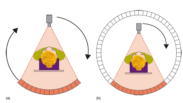
Third – generation type CT scanners use a small array of detectors that are located directly opposite the X- ray source. The detectors rotate so that they are continuously exposed to the X- ray beam. In fourthgeneration scanners, there is a complete ring of stationary detectors, and only the X- ray source rotates (Figure 3.2). With the advent of slip- ring technology, it has become possible to supply the necessary power to the X- ray source continuously as it rotates. This allows the patient to be moved continuously through the aperture as the X- ray beam rotates, producing a helical dataset. This is known as spiral or volume scanning. It has several advantages over sequential scanning, including shorter acquisition times, reduced movement artifact, reduced partial volume artifact, and better reconstruction into coronal, sagittal, and oblique planes.
Figure 3.1 An example of a modern computed tomography scanner, showing the table, head support, and gantry. (With permission from Cardiff University, UK.)
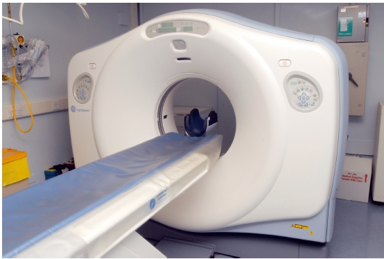
Figure 3.2 Diagrammatic representation of third- and fourth- generation computed tomography scanners. (a) In thirdgeneration scanners, both the X-ray source and detectors rotate around the patient. (b) In fourth- generation scanners, there is a complete ring of detectors and only the X-ray source rotates. (With permission from Cardiff University, UK.)
Multislice CT (MSCT) is a procedure in which 4–16 slices are acquired simultaneously. This has several advantages over conventional CT in that it is fast and offers increased flexibility, including easier 3D reconstructions.13 This high- dose technique should only be considered if there is a significant increase in the expected diagnostic yield.
Low- dose techniques in which either the milliamp è rage to the X- ray tube is reduced or the pitch of the spiral is increased are being developed. The results of these studies are promising, and significant dose reductions can be obtained without any appreciable loss in diagnostic information. This technique has the added advantage over CBCT in that the soft tissues can still be evaluated.14,15
Image reconstruction
The dataset comprises a series of projections that are reconstructed using mathematical algorithms such as the Feldkamp algorithm – a type of filtered back projection.16 With sequential imaging, each slice of data is made up of a matrix of voxels (volume elements). There are typically 512 × 512 voxels in a slice, with the width of each voxel being equivalent to the slice thickness. A voxel in a 2 mm slice would typically be 0.5mm × 0.5mm × 2 mm. The reconstructed image is composed of a matrix of pixels (picture elements). Each individual pixel is assigned a Hounsfield number dependent upon the linear attenuation coefficient at that particular pixel relative to water. This process is shown in Figure 3.3. Typical Hounsfield numbers are shown in Table 3.1.
Figure 3.3 Diagram showing the construction of the image in conventional computed tomography. In this example, a single high- density circular disc is scanned, and the voxel and pixel matrices used are both 10 × 10; the original object is shown on the left (a); the voxel matrix in the middle (b), and the pixel matrix on the right (c). Since at voxel A there will be no attenuation of the beam, it will be displayed black in the final image. At voxel C, the beam is fully attenuated and so is displayed white. At voxel B, the beam is partially attenuated and is displayed mid- gray. In the example, the circle appears very “boxy,” but in reality the matrices are much larger (typically 512 × 512) and would appear round in the final display. (With permission from Cardiff University, UK.)
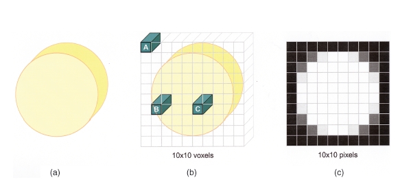
Table 3.1 Table showing the Hounsfield numbers for some of the tissues
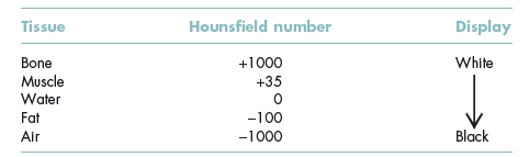
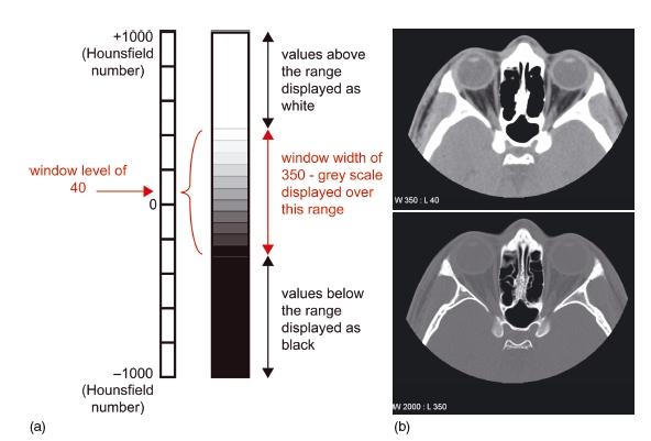
Figure 3.4 In the diagram, typical values for demonstrating soft tissue have been chosen (window level 40, window width 350) (a). Examples are shown of axial images through the orbits displayed on soft tissue windows (window level 40, window width 350) (b, top), and bony windows (window level 350, window width 2000) (b, bottom). Using soft tissue windows, fat, muscles, and the globe are easily distinguished, but the bone is uniformly white with no detail. Using bony windows, the detail within the bone is seen. (With permission from Cardiff University, UK.)
The Hounsfield number given in Table 3.1 for bone is for average bone; for dense compact bone such as the petrous temporal bone, even higher Hounsfield numbers would be assigned.
Before the picture is displayed, it is necessary to “window” the image. This allows the tissues of interest to be displayed over a suitable gray scale. The window level corresponds to the average Hounsfield number of the particular tissue under investigation, and the width is the range of Hounsfield numbers over which the gray scale is displayed. Tissues outside the range are displayed as either white (if the number is higher than the width) or black (if the number is lower than the width). This is shown in Figure 3.4.
Figure 3.5 An axial slice and a three- dimensional reconstruction of the same patient showing marked amalgam artifact. (Courtesy of Mr Michael Fardy.)
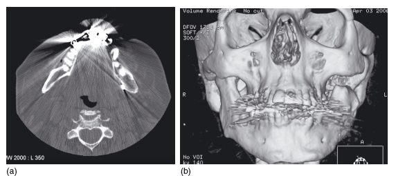
Amalgam can significantly degrade the images, causing “star artifacts” that can greatly decrease the diagnostic yield. This affects both the axial images and also any 3D reconstructions that are planned (Figure 3.5).
3D reconstruction
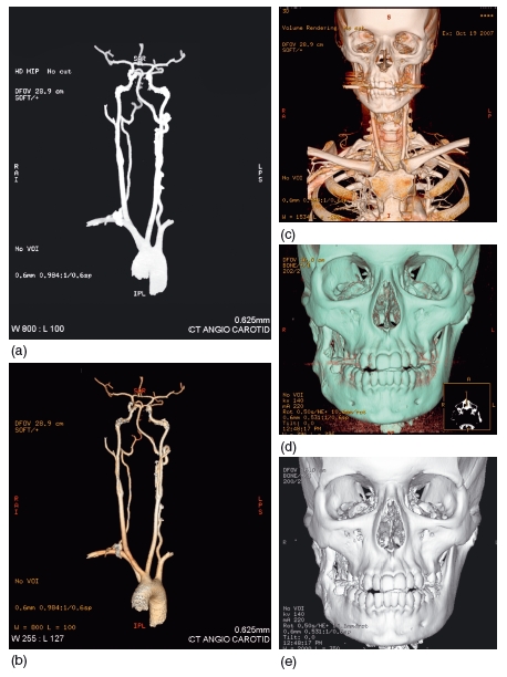
Several types of 3D reconstruction are possible, including maximum -intensity projection, surface rendering, and 3D volume rendering. These are reviewed in an excellent article by Calhoun et al.,17 and it is beyond the scope of this chapter to describe the algorithms utilized to produce the reconstructions. Briefly, however, with a maximum-intensity projection only the voxel with the highest Hounsfield number along the path of the X- ray photon contributes to the density displayed at each pixel. Although the resultant image may appear 3D, this is misleading as no true 3D relationships are displayed. Its main application is in angiography (Figure 3.6).
Surface rendering reconstructs surfaces as if a light is being shone onto the object to produce bright and shadowy areas. The surfaces are chosen by thresholding the data so that only the required surface type is displayed. 3D volume rendering utilizes all the voxels along the ray to ultimately produce the image. High computing power is necessary to perform the appropriate calculations, but it is possible to change the opacity of 3D objects so that underlying structures can be seen. 3D volume rendering is becoming the most useful of these techniques, and the reconstructions can be produced using data generated from CBCT imaging.
Accuracy
The smaller the voxel size, the better the resolution, but as ever there is a trade – off between image quality and radiation dose. Early studies assessing the accuracy of measurements taken from 3D images showed that the methods had to be improved before accurate measurements could be made.18 However, recent studies are much more promising.
Figure 3.6 (a) Maximum-intensity projection of a carotid arteriogram and (b) volume-rendered reconstruction of the same arteriogram. (c) Volume-rendered image showing both the vascular and bony anatomy of the head and neck region. (d) Volume-rendered three- dimensional reconstruction and (e) surface-rendered reconstruction of the same patient. Although the images appear similar, the advantage of volume-rendering is that the translucency of the reconstruction can be altered to see below the bone surface. (Courtesy of Dr Maggie Hourihan.)
In one study, the relative position of the inferior dental canal to the alveolar crest was investigated, and no statistically significant differences were found between 2D CT, 3D CT, and direct measurements.19 However, 2D CT consistently overestimated the distances, and 3D CT underestimated them. In another study, both the precision (reproducibility between two different observers) and the accuracy (validity) of 3D volume- rendered images produced from MSCT data were investigated, this time for linear measurements in the region of the mental foramen. It was found that the linear measurements were both valid and demonstrated a high degree of precision.20
In another cadaver study,21 13 heads were imaged using spiral CT. Linear measurements used in anthropometric analysis were identified in both 2D and 3D. In addition, soft tissue thickness was also measured. The error between the mean actual and the mean 3D linear measurements was 0.83% for bone and 1.78% for soft tissue, with low standard deviations, demonstrating high accuracy for both bone and soft tissue. Overall, these 3D applications are suitable for orthognathic planning.
Quantitative CT has been used extensively in the measurement of bone mineral density (BMD) in the diagnosis of osteoporosis. The advantage of quantitative CT is that the true volumetric density can be measured of either the trabecular or cortical bone at any site, including the jaws.22 CT is considered to be one of the most accurate methods of assessing BMD in the jaws.
Radiation dose
When considering the radiation dose of an investigation, the effective dose is usually cited because it allows comparisons between different radiographic examinations. It takes into account both the type of radiation employed and the radiosensitivity of the tissues irradiated. The effective dose from CT of the mandible ranges from 364 to 1202 μ Sv, and that of the maxilla from 100 to 3324 μSv.23 The marked variation is likely to be due to different scanning parameters employed. When “low- dose” techniques, as described earlier, are used there may be an eightfold decrease in skin dose.24
Clinical applications
CT is extensively used in the evaluation of tumors in the head and neck region. Both primary and metastatic spread may be assessed, with CT and MRI often being complementary in these cases. Iodinated contrast is often used to help delineate normal anatomy from disease and to investigate vascular anomalies.
Because CT is well suited to visualizing bone morphology in 3D, it has been used extensively to assess facial asymmetry. 25 Although there can be difficulty in finding landmarks that are not affected by deformity, the external auditory meatus may be considered as a suitable reference landmark.26 With regard to a stable reference plane, the Frankfort horizontal plane has been suggested.27 3D volumetric data may be used to produce 3D cephalographs. The traditional landmarks used on 2D cephalometry may also be placed in 3D to allow a true global assessment of the patient.28 It is interesting that the landmarks on the 2D cephalograph are often imprecise and may not reflect the actual position of these structures on the 3D reconstructions (Figure 3.7).
In patients with clefts of the maxillary alveolus, it is important that sufficient bone is grafted into the cleft to allow spontaneous eruption of the canine into the dental arch. CT has been used to preoperatively assess the volume of grafted bone required.29,30 3D CT will also show the spatial relationship of the unerupted teeth so an assessment of likely spontaneous eruption can be made. Overall, CT seems to give a better assessment of outcome than conventional radiography,31 but it should only be used in selected cases. CT has also been used to evaluate secondary bone grafting.30,32 Resorption of the graft seems more likely if teeth are absent or if orthodontic intervention is necessary to align the teeth.30
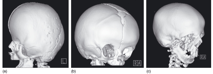
3D CT reconstructions have been used to assess craniofacial disorders such as Apert and Treacher Collins syndromes. It aids confirmation of the diagnosis and helps in detailing the sutures and synostoses.33 Examples of these conditions are shown in Figure 3.8. Movement artifacts can be problematic as the patients are often very young when they are scanned, but this may be reduced using MSCT. Since only a limited amount of the cranium can be scanned using CBCT, it is unlikely that this modality will help, particularly if the abnormality involves the posterior cranium.
Figure 3.7 The points are placed on the lateral cephalogram (far left), and these points are projected onto the three- dimensional model. The points on the three- dimensional model do not coincide with the midline points A and B and pogonion (Pg). The postnasal spine (PNS) marked on the radiograph is 8 mm in front of the real PNS. In this example, a cone beam computed tomography scan has been used to generate the three- dimensional model (Maxilim ©, Medicim NV, Belgium).
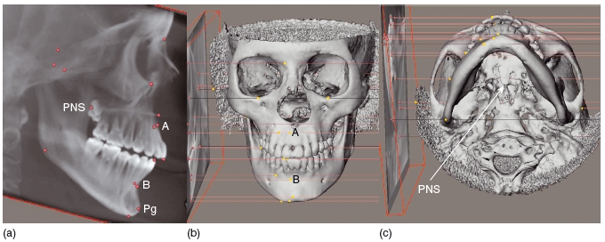
Figure 3.8 Three- dimensional reconstructions of craniofacial disorders. (a) Apert syndrome, showing an elongated or tower- shaped skull due to craniostenosis. (b) Craniosynostosis, following premature closure (synostosis) of the right coronal suture. (c) Treacher Collins syndrome with absence of the zygoma. (With permission from Dr Helen Williams, Birmingham Children’ s Hospital, UK.)
CT has also been recommended prior to bilateral sagittal split osteotomies to help identify the mandibular canal, as it is superior to conventional spiral tomography in locating this structure. However, CT is not necessary for all patients, although it may prove useful in those with a thin ramus or with marked facial asymmetry.34
Several software programs have been developed that allow the planning of osteotomies in 3D. These allow trial bone cuts and bone movements to be made and alert the operator if the proposed movements of the jaws are not possible or are likely to cause collision between adjacent anatomic structures.35 These programs can also be used to predict the final bony and soft tissue profiles, which may prove extremely useful in planning complicated orthognathic surgery.36 Similar programs may also be used when planning distraction osteogenesis. The 3D data are imported into the software, and the proposed cuts in the bone are made “virtually” on the 3D model. The fragments are then moved into the proposed position. From this, a vector is calculated so that a suitable design of distraction device is used and is correctly positioned.35 Vectors may also be calculated on a rapid prototyping model,37 and both techniques appear to be comparable.38
In addition, 3D data from CT scans can be used to produce a virtual set- up of the teeth within the dental arch. This process merges the CT data with data from the laser – scanned study models. This allows the operator to assess the relationship of the teeth to the bone before treatment and also assess the degree of fenestration of bone that may be present following planned tooth movements.39 Similar multimodal fusion techniques have also been used for planning orthognathic surgery. The technique of merging CT data with the laser- scanned study models allows the post- surgical relationships of the teeth and jaws to be realized virtually and allows quantification of the desired surgical movements to produce the optimum result (Figure 3.9).40
Double- CT techniques combining CT scans of the jaws and CT scans of the study models have also been suggested to produce the virtual model of the teeth and jaws.41 However, at present, laser scanning has been shown to be superior to CT in its accuracy of depicting the study casts.42 It is also possible to use volume- rendered MRI scans in some orthognathic planning software programs.
CT has been extensively used to examine the bony aspect of the temporomandibular joint (TMJ). It is used to evaluate trauma (Figure 3.10) and bony neoplasms, and has been shown to be accurate in assessing the condyle and mandibular fossa in patients with rheumatoid arthritis.43
CT is the imaging modality of choice for imaging complex or severe maxillofacial trauma (Figure 3.11). Often surgical landmarks are difficult to identify on axial slices, and 3D reconstructions help with their accurate identification.44,45 It has also been used in the assessment of the volume of bone necessary to graft traumatic defects.46 In addition, rapid prototype models may also be constructed to aid diagnosis and treatment planning (Figure 3.12).
CBCT, or digital volume tomography, is an exciting new development in the field of maxillofacial radiology. However, its use in medical imaging is not new as these systems were already being used in vascular imaging and radiotherapy planning. The first commercially available CBCT scanner, the NewTom- 9000 (Quantitative Radiology, Verona, Italy) was produced in 1996. Since then, many of the major manufacturers of dental imaging equipment have produced or are developing CBCT units specifically for imaging the teeth and the maxillofacial skeleton.
The machines are significantly cheaper than conventional CT machines, principally because the X- ray tube used has a much lower heat capacity and the technology used is less complex.47 The detectors comprise either an image intensifier linked to a charge- coupled device, or an amorphous silicon flatpanel detector consisting of a caesium iodide scintillation screen and photosensor array.48 The machines are generally smaller than conventional CT machines. Superficially, some may look very similar to conventional CT scanners, but no moving gantry is employed and the table does not move through the aperture. However, most machines resemble panoramic machines, with the patient either sitting or standing upright (Figure 3.13).
Figure 3.9 Three- dimensional segmentation of the mandible and maxillary teeth (top). The scan data are fused to data obtained from three- dimensional laser scanning of the mandibular and maxillary study casts in order to plan orthognathic surgery (bottom).
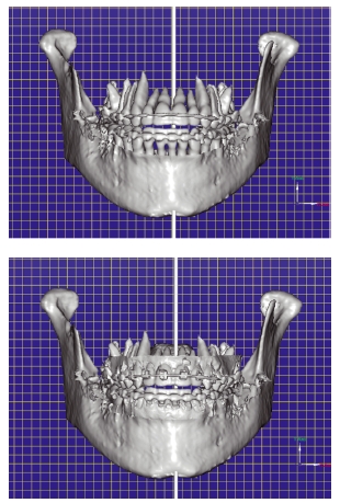
Figure 3.10 Axial slice (a) and three- dimensional reconstruction (b) through the left temporomandibular joint showing an abnormally shaped condyle that had previously been fractured. The condylar head had been displaced medially following the original traumatic episode. (Courtesy of Mr Michael Fardy.)
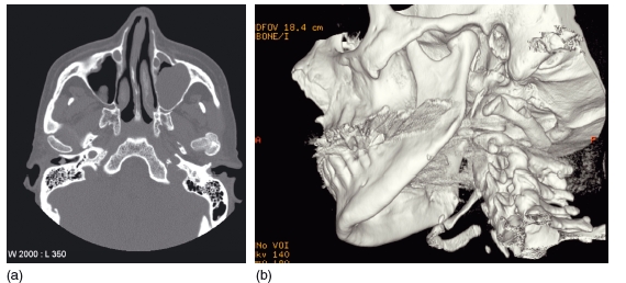
Figure 3.11 Three- dimensional computed tomography reconstruction showing multiple fractures of the mandible including a comminuted fracture of the right body. (Courtesy of Mr Andrew Cronin.)
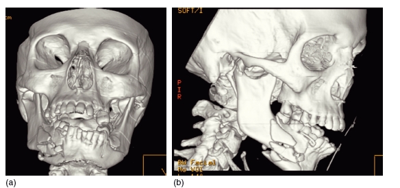
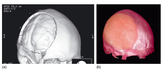
Figure 3.12 Three- dimensional reconstruction of the skull. This shows a defect in the skull following a decompression craniectomy (a). The data from this have been used to construct a rapid prototype model. The defect has been filled in with wax, and from this a titanium plate can be constructed to repair the surgical defect (b). (Courtesy of Mr Andrew Cronin.)
The patient is positioned using laser beam markers to ensure they are centred correctly within the machine (Figure 3.14). A cone shaped X- ray beam is utilized, and during a single rotation of the X- ray source and detector around the patient, a series of 2D projections is obtained. This process is illustrated in Figures 3.15 and 3.16. For a “standard” scan using the Classic i- CAT (Imaging Sciences International, Hatfield, PA, USA), 306 projections are acquired, but if a higher resolution is required 599 projections are obtained. The data from these projections are reconstructed using sophisticated algorithms similar to those used in conventional CT to produce a volumetric dataset.
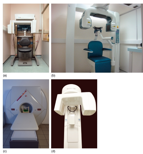
Figure 3.13 Examples of cone beam computed tomography units. (a) The Classic i- CAT (With permission from Imaging Sciences International, Hatfield, PA, USA and Cardiff University, UK). (b) The 3D Accuitomo (J. Morita Mfg. Corp., Kyoto, Japan). (With permission from the manufacturer (GmbH), courtesy of Eric Whaites, Department of Dental and Maxillofacial Radiological Imaging, King’ s College London, UK.) (c) The NewTom 3G (QR srl, Verona, Italy). (With permission from QR srl (Quantitative Radiology).) (d) The NewTom VGi (QR srl, Verona, Italy). (With permission from QR srl (Quantitative Radiology).)
This process, known as primary reconstruction, can take several minutes to perform and is partly dependent upon the number of projections obtained and the processing power of the PC used. Secondary reconstruction is, however, extremely fast and generally results in images in the axial, coronal, and sagittal planes (Figure 3.17). In addition, multiplanar reformatting into other clinically useful planes is also possible. These include panoramic type views, cross- sections through the jaws, and corrected lateral views of the TMJ.
Figure 3.14 Correct positioning of the patient for cone beam computed tomography scanning is attained using a series of laser beam markers and stabilization aids such as a chin cup. (With thanks to Nicola O’ Kelly.)
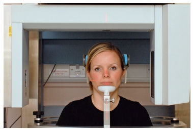
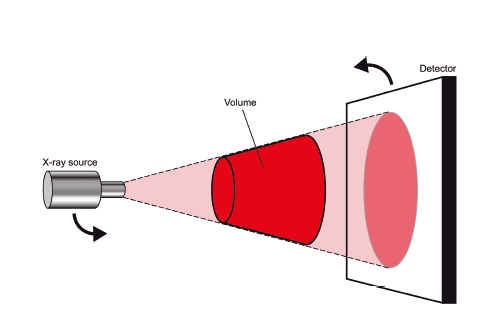
Figure 3.15 Diagram showing the cone shaped X-ray beam used in cone beam computed tomography. A single rotation of both the X-ray source and the detector around the patient produces the “volume of interest,” which can then be reconstructed. (With permission from Cardiff University, UK.)
Although the reconstruction time is quite long, the scanning time is quick (10–40 seconds), which is an advantage, particularly when scanning children, as it helps to reduce the chance of movement artifacts. Paradoxically, movement artifacts are more common with CBCT than with conventional CT. 49 Stabilization aids such as biteblocks, chin cups, and head straps may help reduce movement, but their use can alter the soft tissue morphology, which can be an important consideration.
Diagnostic Imaging 43
Figure 3.16 During the rotation, a series of projections is obtained. In this illustration, eight projections are shown, although in reality several hundred are acquired. The photographs show the view of the patient “as seen” from the X-ray source, along with the resultant projection image. (With permission from Cardiff University, UK, and thanks to Nicola O’ Kelly. Projections used with permission from Imaging Sciences International.)
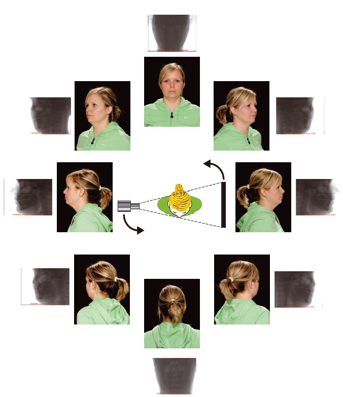
Figure 3.17 Example of a secondary reconstruction into axial, coronal, and sagittal planes. The green, red, and yellow lines allow easy cross-referencing between images. (With permission from Imaging Sciences International.)
There are three categories of CBCT scanner: large field of view (FOV), medium FOV, and small FOV scanners.50 The large -volume scanners are capable of scanning the whole facial skeleton, the medium-volume ones are used to scan both jaws together, whereas the small-volume scanners are well suited for imaging single jaws, small sections of the facial skeleton, and small groups of teeth. Therefore the clinical applications for these machines are different. The differences between the machines are becoming less distinct as several manufacturers now produce machines that will perform scans using all three FOVs.
Performance and accuracy
CBCT shows the bone and teeth well, but amalgam produces artifact that can degrade the image, although this is often less severe than with conventional CT (Figure 3.18).49
Spatial resolution – the ability to distinguish two structures close together
The voxels within the volume recorded are isotropic (cubic) and can be much smaller than conventional CT, in the range 0.125 – 0.4 mm3. These features help to ensure excellent spatial resolution in all planes. The spatial resolution for the small- volume units is over two line- pairs per millimeter (at 10%), and may become as high as four line- pairs per millimeter in the near future. In practical terms, if a voxel size of 0.2 mm is chosen in the scanning parameters, high- contrast objects 0.4 mm or greater in size should be detected. The resolution is dependent on the scan parameters selected (time, milliamp è rage, and kilovoltage), as well as the construction voxel used (Figure 3.19).
Figure 3.18 Axial (a) and sagittal (b) sections through the maxillary teeth. The amalgam restorations in the upper right first and second molars cause less severe artifacts than on conventional computed tomography. However, they do cause a radiolucent artifact in the adjacent teeth that can mimic dental caries. (With permission from Imaging Sciences International.)
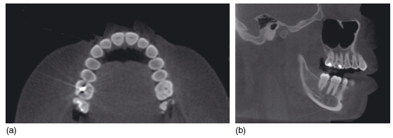
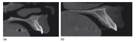
Figure 3.19 Sagittal reconstructions though the incisor region (of different patients). Image (a) was obtained with a longer exposure (more projections obtained) and reconstructed using a 0.2 mm voxel size, and the image appears sharp. Image (b) was obtained using a shorter exposure time (fewer projections obtained) and reconstructed using a larger voxel size. The resultant image appears less sharp, but at a lower dose to the patient. (With permission from Imaging Sciences International.)
Contrast resolution – the ability to distinguish adjacent structures that have only small differences in density
Cone beam systems have low contrast resolution, and it is therefore not possible to differentiate between the soft tissue structures (Figure 3.20). Although this is a limitation of these systems, it should be remembered that these machines were designed specifically to image the hard tissues.
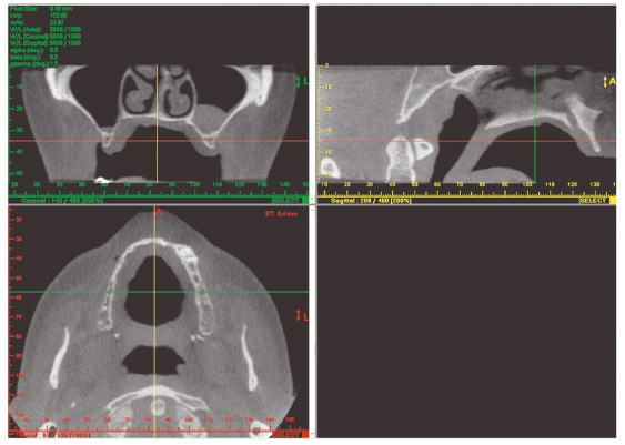
Figure 3.20 Axial section through the orbital region. The bone is shown well, but there is poor differentiation of the soft tissues. Compare this image with Figure 3.4 (conventional computed tomography), in which all the various soft tissue types can be identified. (With />
Stay updated, free dental videos. Join our Telegram channel
VIDEdental - Online dental courses


