In dentistry, metal alloys are widely used because pure metallic elements are very limited in terms of strength and stiffness. Alloying allows a much wider range of properties for two reasons: one, the types and detail of crystal structure can be modified over very wide ranges; two, metals containing more than one type of structure can be created. Constitutional diagrams can be read to interpret the structures in alloys as a preparation for the study of dental alloys. In particular, the expected effects of variation in temperature and composition can be determined directly.

Only under special circumstances do alloys exhibit sharp melting points. Ordinarily, solidification leads to non-equilibrium structures in which the components are segregated. This is nearly always a bad thing in that very weak regions may be present, corrosion is enhanced, and the structure is prone to change with time or heating.

When complete solid solutions of one metal in another are not possible, more than one phase may be present at equilibrium. In the simplest case, this leads to a eutectic type of system in which a minimum melting temperature is observed. The freezing behaviour, and the types of structure to be found, are characteristic.

Although metal phases often have very wide composition ranges, metal alloy systems produce intermetallic compounds in which the composition is more narrowly defined. Despite this, even the more complicated constitutional diagrams can all be read in the same way, allowing descriptions of the effects of changing overall composition and the reactions that result from heating and cooling, whether these reactions are solid-liquid or completely solid state.

The scope of dental alloys is very broad and ranges from amalgam fillings to gold for inlays, from cobalt-chrome for bridges to stainless steel for appliances. Discussion of the behaviour of these and other systems requires reference to phase diagrams. Understanding dental applications is therefore dependent on a grasp of the fundamentals.

The properties and behaviour of metals have been described in the previous chapter in terms of atomic- and grain-scale structure. There are however effects on a further level, those directly due to the presence of alloying elements. Apart from the crystal disorder introduced by their presence in solid solution, the melting and freezing of alloys differ from these processes in pure systems, and compositional and structural effects follow. Since alloys are far more varied and useful than pure metals in general, we must consider these effects of alloying in order to understand the properties of the alloys. In so doing, some of the rules for reading phase diagrams will be elucidated, rules which apply in many systems, not just metallic ones.

Gases, it will be recalled, mix freely with one another in all proportions (that is, assuming no chemical reactions). The mixture will be thoroughly homogeneous, each kind of gas molecule being distributed randomly throughout the space available. Liquids, too, may exhibit complete miscibility in all proportions, such as with ethanol and water, but equally may show two layers or phases. An example of this latter type of case would be chloroform and water. In such combinations each liquid is apparently totally insoluble in the other. More usually, each liquid shows some degree of solubility in the other. Each such phase may then be referred to as a solution, which must of course be saturated with respect to the other component if the other solution phase is in contact with it at equilibrium. A phase diagram can be used to show the variation of solubility with temperature, and examples are readily found in physical chemistry textbooks. Similarly, a composition-temperature phase diagram can portray a system consisting of a solid and a liquid in which it is soluble (sugar and water) for example. The liquid consists of an entirely homogeneous random dispersion of sugar molecules in the water, but the solid (in this case, at least) contains no water.

These ideas concerning solution are relevant also in the solid state: within the limitations of chemical similarity, lack of reaction and radius ratio (11§3.7), atoms of one metal may be mixed with those of another, one metal dissolved in another, with the implications of randomness of lattice site occupied and homogeneity. This is solid solution. The complete range between totally insoluble, through limited mutual solubility, up to complete solid solubility in all proportions may be observed.

•1.2 Continuous solid solution

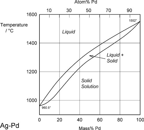
Two examples of complete solid solubility were introduced in 11§3.7, namely Ag-Au and Ag-Pd. Their phase diagrams are shown in Figs 1.1 and 1.2. Two points are of immediate interest. Firstly, it can be seen that, below the melting point of Ag, there is a complete absence of structural change as the one element is dissolved in the other, that is changing composition from one extreme to the other (depending on the point of view, or from which side of the diagram one works). Indeed, there is only one all-solid phase field, and this only contains one phase. Such a system is known as a continuous solid solution. Secondly, there is now a new kind of region to consider, one that lies between (all) Liquid and (all) Solid. This region corresponds to the presence of both states simultaneously, at equilibrium. The upper and lower boundaries of this region are known as the liquidus and solidus respectively (Fig. 1.1) (and are taken by convention to themselves represent the presence of two phases). The key point is that there is a temperature difference between these two lines at any composition except for the pure metals, when the lines coincide. The complications of alloy metallurgy arise from precisely this kind of feature in a phase diagram, and the effects of changing the temperature of a mixture through such a phase field is what we shall now discuss.

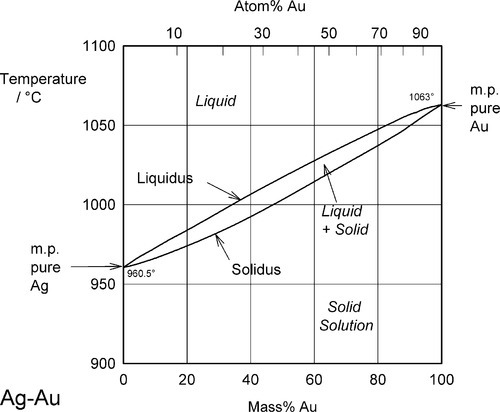
Note the characteristic pattern of phase field boundaries at the left- and right-hand boundaries, the terminals. There is a K-shape, a sideways ‘V’, < or >, formed by the liquidus and solidus meeting at the point where they touch the vertical boundary. In addition, note the occupancy of or number of phases in the phase fields around this point: 1,2,1 – liquid, solid + liquid, solid. This is a universal pattern.

•1.3 Partition

To understand the implications of this kind of pattern, and one of the ways phase diagrams may be interpreted, we proceed with another thought experiment. So, starting at low temperature somewhere in the all-solid phase field, and raising the temperature, no structural change is to be observed so long as we remain in that solid solution region. But at some point the solidus will be reached, and melting will commence. We now have two phases in contact; both are solutions, but in different states. These states are distinguished by the presence or absence of long range order. In other words, they are solid and liquid. However, the chemical potentials of each of the components will have changed in going from a solid to a liquid of the same composition, and changed (in general) by different amounts. However, for a system to be in equilibrium it is required that the chemical potential of any element is the same in all phases which are then present (8§3).

Thus, for a given component in the just-melting system, the chemical potential will be different in the two kinds of environment. It will then adjust its concentration in the two phases, by diffusion one way or the other across the boundary, until the potential is equilibrated (and there is no further driving force for change). In other words, that component will partition itself between the two phases until that thermodynamic requirement is met (cf. the effect of temperature discussed in 8§3.2). This must occur simultaneously for all components present. Consequently, the compositions of the solid and liquid in contact at any temperature at equilibrium will differ. Clearly, if this is the case, one phase must become richer in one component and poorer in the other, and vice versa, since the overall composition is fixed. As with all processes this kinetic activity depends on the availability of the activation energy for the process, and the time for it to occur. We shall for the time being assume perfect equilibrium at all stages.

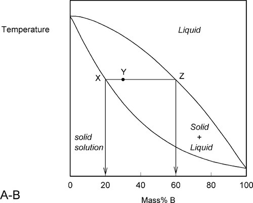
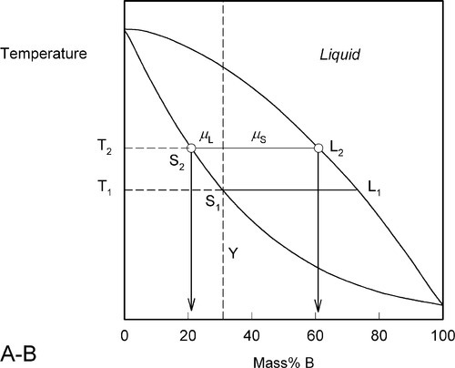
A stylized diagram of the continuous solid solution type for just such a system is shown in Fig. 1.3. If we consider a typical isothermal tie-line XZ, its ends are, by definition, at the solidus and liquidus. Consequently, at an overall composition corresponding to X, and at that tie-line’s temperature, there would be solid having the corresponding composition (in this example, 20% B) in equilibrium with an infinitesimal amount of liquid (lever rule, 8§3.10). Similarly, at an overall composition corresponding to Z, liquid with the corresponding composition (i.e. 60% B) is in equilibrium with an infinitesimal amount of solid of composition corresponding to X. To reiterate the point: since it is an isothermal tie-line, and both points represent solid-liquid equilibrium, and are in the same phase field, both solid and liquid must have the same individual compositions at the two points. In other words, at both X and Z, the solid has the composition X and the liquid has the composition Z. This must also be true for any other overall composition point in between, such as at Y. This principle of the interpretation of isothermal tie-lines within a two-phase field is perfectly general for two-component systems. Indeed, in a sense, this is the embodiment of the thermodynamic demands of equilibrium.

•1.4 Heating

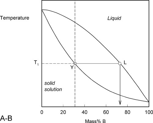
We now proceed to raise very slowly the temperature of the system with the overall composition corresponding to Y in Fig. 1.3, i.e. about 31% B (Fig. 1.4). When the solidus is reached, at T₁, the first infinitesimal amount of liquid, of composition corresponding to L (i.e. richer in B than is solid Y) has appeared. The solid composition is hardly affected because the amount of liquid is so small. It is still just about 100% solid that is present.

Heating a bit further, to T₂, and allowing the system to come to equilibrium, we now have a solid corresponding to S₂ (approximately 21% B) coexisting stably with a liquid of composition corresponding to point L₂ (approximately 61% B) (Fig. 1.5). In other words, S₂ has a larger proportion of A than the overall composition Y; while L₂ is richer in B than Y, it is in fact richer in A than L₁, the first liquid to have formed. The amounts of liquid and solid are in the mass proportions μ_L : μ_S according to the corresponding line segment lengths of the tie-line. What has happened is that in going to temperature T₂ more atoms of B have left the solid surface than of A, leaving that surface richer in A. These A atoms then have diffused (slowly) into the solid so that it is of uniform composition throughout. The system continues this slow dynamic adjustment until the equilibrium situation is attained.

This process continues on further heating to a temperature such as T₃ (Fig. 1.6), making the solid (S₃) richer and richer in A while the liquid (L₃) does the same (but not necessarily at the same rate, it depends on the slopes of the liquidus and solidus at any given temperature). Of course, as melting is occurring, there is proportionately more liquid and the ratio μ_L : μ_S is now larger.

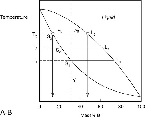
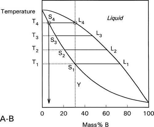
These changes occur progressively until the liquidus is reached (Fig. 1.7). At this point, T₄, only an infinitesimal amount of solid remains, with composition corresponding to S₄, while the liquid L₄ is now just the same as the original overall composition Y. This is reasonable when (very nearly) all original solid has melted. Beyond that temperature there is no further phase or composition change.

This kind of analysis is on the assumption that complete equilibrium can be maintained at every stage, which means allowing time for diffusion in the solid, such diffusion being the rate-limiting step. The overall composition is of course guaranteed to be constant by mass balance. For such a system it is only at pure A and pure B that the liquid can have the same composition as the solid at equilibrium.

•1.5 Cooling

The converse process can be traced just as simply by taking the figures in the reverse order. Thus, taking the overall composition Y again, and starting in the melt, the first solid to appear has the composition corresponding to S₄. As cooling progresses the solid becomes richer in B: S₄ – S₃ – S₂ – S₁ (which last is identical to the overall composition), while the liquid also does: L₄ – L₃ – L₂ – L₁. The proportion of liquid to solid, μ_L : μ_S gradually declining to zero at the solidus temperature of Y.

•1.6 Segregation

Now the accuracy of all of this depends ultimately on the equilibrium of all of the solid with the liquid at every step of the sequence, whether in heating or cooling. But because during cooling successively-formed solid will be in layers on earlier already-formed grains, so equilibration tends to be inhibited because the diffusion rate in the solid state is less than in the liquid state by a factor of about 10^– 4. So the assumption made in §1.3 is now abandoned as unrealistic. In effect, those atoms which do not belong in the solid at the current temperature are trapped because the rate of advancement of the solidification front is faster than they can diffuse. Consequently, in practice the composition of the solid changes steadily from the nucleus of each crystal out to the grain boundary, becoming steadily richer in the lower melting component. If this is occurring the effective overall composition of the solidification system will drift towards pure B, as A is made unavailable by being locked-up or sequestered inside the earlier-freezing solid. In this way the last solid to form may have a composition closely approaching pure B.

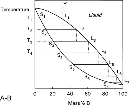
The process can be imagined as occurring in a stepwise cooling sequence. In Fig. 1.8, the first solid to form on cooling from Y to T₁ has the composition corresponding to S₁. If we now jump to T₂, the solid which forms corresponds to S₂, which leaves the liquid with the composition of L₂. Since equilibration is not occurring it is now that liquid L₂ which on cooling to T₃ starts to freeze, so that the next solid to form corresponds to S₃, leaving liquid L₃. It is then this liquid that is cooled to T₄, producing solid S₄, leaving L₄ – and so on. It can be seen that this ultimately leads to the final tiny amount of liquid to freeze being essentially pure B. This is the case no matter how small the cooling steps are. In other words, even continuous smooth cooling results in a non-equilibrium, layered or gradient structure (Fig. 1.9).

This is the process of segregation: the variation in composition from point to point in the solid when homogeneity was expected. The structure is now said to be cored. It usually requires extensive annealing at a temperature high enough for diffusion to occur readily (and yet below the solidus or any other transition) for an equilibrium structure to be formed eventually; this is homogenization. It is a seeming paradox that, up to a point, the slower the cooling rate the further from equilibrium the phase description and phase compositions may be. But the faster is the rate of cooling the less material will actually freeze out at a particular temperature; there is a kinetic limitation to local equilibration. This is in effect supercooling, but instead of the temperature rising of necessity back up to the melting point as with a pure metal and establishing equilibrium, the composition of the then solidifying metal will have the composition corresponding to that indicated by the tie-line at that temperature (but only because the rate of loss of heat is so great). The last metal to solidify will have a composition closer to the overall composition, and the cast ingot would require relatively little annealing to redistribute the components (by diffusion) to achieve an equilibrium structure.

Fast cooling like this is referred to as quenching, the intention being to try to prevent the segregation referred to above, or at least to reduce it markedly, by not permitting time for the required diffusion to occur. Liquid is solidified at close to its overall composition. In addition, the effective supercooling produces a large number of crystallization nuclei, and so the average crystal (grain) size will be small. This makes the distances over which diffusion will be required for subsequent equilibration correspondingly small, and the required annealing time short, even if the segregation is marked.

It is worth stressing that the outcome of the solidification of a melt is dependent on two equilibration systems: liquid with fresh solid, and that fresh solid with underlying material. In effect, the diffusion rate of atoms in the melt is so high that under most ordinary circumstances it can be considered as nearly homogeneous, no matter what the composition is of the solid currently forming. Thus, that solid can be treated as if formed in equilibrium with the current liquid composition, as dictated by the tie-line: exchange of atoms between liquid and solid surface is rapid. Exchange between any pair of layers in the solid, including the outermost, depends on solid state diffusion, via vacancies, which may be ten thousand times slower. However, this view does suggest that if the cooling rate is fast enough, equilibration at the liquid interface cannot occur and the composition of the solid that forms is closer to that of the liquid, which therefore does not show as much drift in composition over the whole process. However, extremely high cooling rates simply cannot be attained if the thickness of the metal is too great (more than a few tenths of a millimetre) because thermal conductivity then becomes the limiting factor. Nevertheless, such cooling rates may be achieved (or approached, at least) for the layer of metal in contact with a cool wall when the melt is poured into a mould, i.e. in a casting. The constitution and grain size of the surface may then differ from the bulk, which is obliged to cool rather more slowly.

The nature of segregation is such that impurities in the alloy, elements that were not intended to be there but that are present in small quantities, and that have low solid-solubility in the main phase(s), will tend to remain in the melt until the very end of solidification as the partitioning is given time to occur. This means that these impurities tend to be concentrated at the grain boundaries, with various potential consequences. They may lead to weaker-than-expected grain boundaries and thus lower strength overall by allowing intergranular cracking to proceed more readily. The composition difference may also allow intergranular corrosion to occur more readily, because of the dissimilar phases now present (13§4.10).

•1.7 Cooling curves

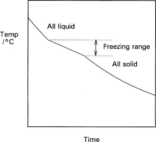
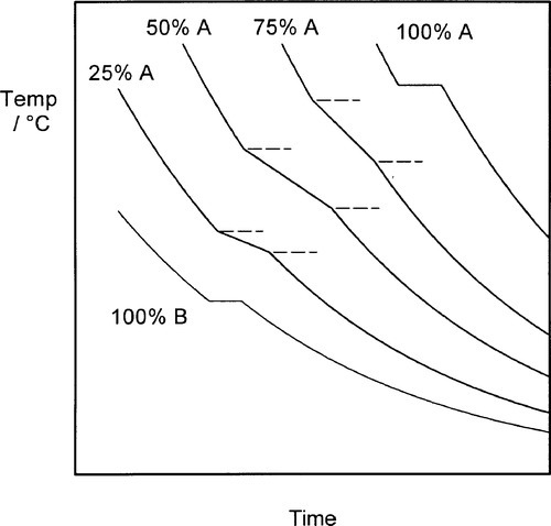
The cooling curve (11§2.7) for a continuous solid solution system should appear as in Fig. 1.10, i.e. with a freezing or solidification range, because the effective freezing point is varying continuously, just as the composition of the equilibrium solid varies continuously. Note that the freezing range corresponds to those temperatures where liquid and solid are coexisting. So for a series of alloys in an A-B, binary, system (Fig. 1.3), a series of cooling curves (Fig. 1.11) will be obtained. From data such as these the phase diagram itself (Fig. 1.3) would be constructed, plotting the temperatures where discontinuous changes in the slope of the cooling curve are found against composition, although usually this approach must be supplemented by metallography – direct observation of grain structure. The difficulty is, of course, that the lower limit of the freezing range can be very uncertain because of the difficulties arising from segregation. However, as mentioned above, for moderate rates of cooling (i.e. not too slow) a better approach to the expected condition can be obtained and cooling curves are often a practical means of obtaining such data in a preliminary way.

One consequence of segregation that is worth noting relates to the experimentally-observed freezing range. While the liquidus will be determined quite accurately, the solidus temperature will not correspond to the end of the freezing range. The last liquid is necessarily of lower freezing point than the solidus for the equilibrium constitution at the given overall composition. The slower the cooling, the worse this might be. Thus, depending on the alloy system, such values from a cooling curve experiment need to be interpreted carefully.

§2 Metallography

One of the approaches which may be taken in determining the actual constitution of a sample of a metal is simply to look at it: metallographic examination. In practice this requires an optical microscope, but this is really only because grain sizes ordinarily are in the range of one to a few hundred micrometres.

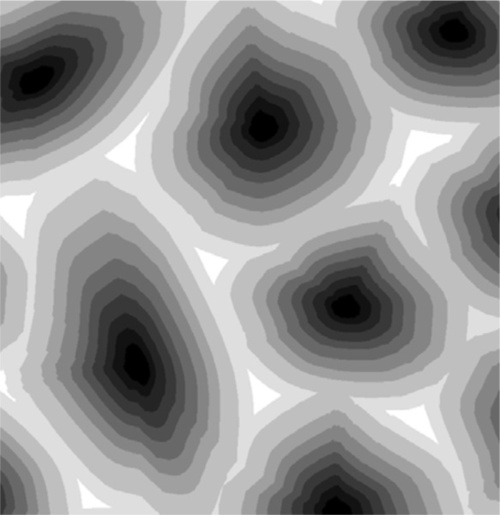
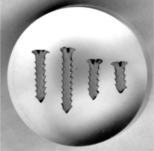
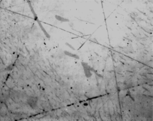
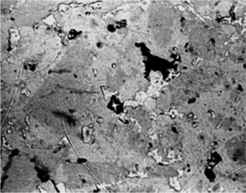
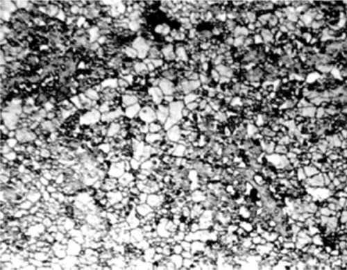
The technique in principle is very straightforward. A specimen of the metal, which may be anything from a very thin foil, through wires, to large objects such as a piece of a casting, is first usually embedded in a block of resin (such as cold-cure acrylic) to facilitate handling. One face is then ground away flat to expose a section of the specimen (Fig. 2.1), using a very coarse grinder or perhaps a saw followed by abrasive paper of decreasing coarseness. Then, using a succession of abrasives such as alumina and diamond dust, the cut surface is polished so that no scratches remain visible (< ~ 0.2 μm), taking care to keep it flat. Sometimes this is sufficient because the phases present have sufficiently different colours that they can be distinguished at this stage (Fig. 2.2). Or, if the hardnesses of the phases differ sufficiently, one or more may be removed more quickly than the surroundings, giving relief effects that show up clearly under the microscope (which must, of course, use reflected light rather than transmitted as with biological sections) (Fig. 2.3).

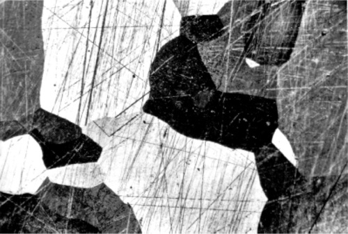
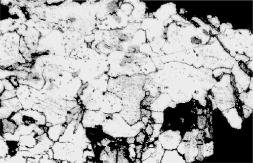
Normally, however, these effects are too weak to give clear images, and etching is used. Metals vary in the rate in which they dissolve in acids, while some develop oxide coats under oxidizing conditions, some dissolve in alkali, and some are extremely resistant. Sometimes a treatment such as this produces a variety of colours, sometimes it simply leaves holes, sometimes it makes the surface rough and therefore dark because it scatters light. Taking advantage of these variations in reactivity, treatment with carefully chosen solutions, at particular temperatures, or carefully timed, can yield striking pictures of the distribution of all of the phases present (Fig. 2.4). These can have different colours or shades (from the deposition of reaction products – tarnished), and clearly defined boundaries, even between grains of the same phase because crystal lattice orientation differs (and therefore reactivity) (Fig. 2.5). Notice how scratches are differentially-enhanced according to the crystal planes they expose. Finally, grain boundaries, because they are disordered and therefore of higher energy than the adjacent crystalline region, tend to react more readily, often leaving a minute groove between grains, which feature is then clearly visible under the microscope (Fig. 2.6).

Of course, none of this on its own identifies a phase or its composition. Series of alloys must be prepared, covering the possible range of compositions at small intervals. These may then be held at a series of known temperatures for long periods to allow the structure to equilibrate, followed by rapid quenching to room temperature to preserve the structure. Metallographic examination then permits the phases to be counted, estimates of their proportions made, and characteristics such as colour or etching behaviour to be noted. Correlation of this data with cooling curve information then permits the building of the constitutional diagram.

In addition, X-ray diffraction is used to determine crystal structure. Unknowns can frequently be identified simply by referring to an index of diffraction data (Fig. 2.7) noting the positions and relative intensitie/>