Metallic alloys, and a few pure metals, are used in many dental procedures. From the stainless steel of hand instruments, through cast gold devices and amalgam to titanium implants, the special properties of metals (such as their strength and ease of fabrication in complex shapes) have been advantageous and will continue to be so. Indeed, they permit dental procedures not otherwise possible. However, in addition to the wide range of properties shown by the metallic elements themselves, by the means of suitable treatment and alloying an enormous range of combinations of properties are possible. This range is so broad that it allows the design of alloys – as opposed to mere passive acceptance of what is already known – for specific purposes with definite values of the necessary properties. How this comes about can be understood from a study of the structure of metals from the atomic scale up to that of the most characteristic entity of metals, the grain, and then how the assemblage of grains behaves in the bulk metal, whether wrought or cast.

The scope is so enormous that new alloys continue to be invented and added to the already huge catalogue. Even in dentistry this process continues, especially for casting alloys, but also for orthodontic and implant use. However, it is not necessary to go into great design detail to understand the dentally-important systems, but it is important to understand basic structural matters and behaviour in order to make effective product selection, as well as to handle metallic materials and devices – including fabrication and finishing – to the best advantage of both dentist and patient.

Metals are essentially distinguished from other types of substance (in the condensed states, solid or liquid) by their special type of bonding. This is known simply as metallic bonding although, as will be seen, it also occurs in substances not usually considered to be metallic. Metallic bonding means that the valence electrons (that is, the ‘outermost’ electrons that are normally involved in chemical reactions) are not confined to specific atom-atom bonds or molecular orbitals but are each spread over all possible sites, that is to say that they are completely delocalized over the entire object, as well as being mobile. There are no underlying directional bonds in true metals.

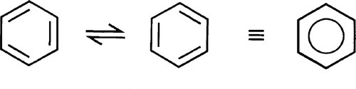
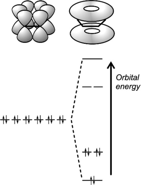
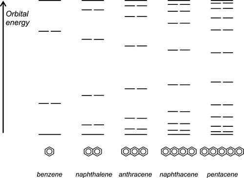
Delocalized electrons will be familiar in the context of conjugated π-bonds in organic chemistry. Thus, in benzene (Fig. 1.1) three double bonds can be viewed as resonating between two arrangements, and the structure overall may be considered as a hybrid of the two. The theoretical picture is of overlap of all of the atomic orbitals to give one molecular orbital (Fig. 1.2). As more and more rings are added to the structure, as in the series naphthalene to pentacene (Fig. 1.3), so the delocalization is greater and the number of energy levels available for the electrons increases, becoming closer together in the process.^[1]

•1.2 Graphite

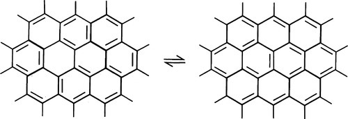
In the ultimate planar carbon ring system of graphite (Fig. 1.4) the number of possibilities of ‘double bond layout’ becomes astronomical. The electrons are then spread over the whole planar network, with very many energy levels available, very close together. Promotion of an electron to a higher level is thus very easy (i.e. requires little extra energy, thermal energies are more than enough), and this leads to the good electrical conductivity of graphite: it is some 100 times greater in the plane of the rings than across them.

The delocalization in graphite is, however, restricted to one plane. The bonding between layers is very weak, being due to van der Waals forces only, allowing the layers to slide past each other easily. This confers the familiar dry lubricating properties of graphite (as well as its usefulness in ordinary pencils: its name comes from the Greek γραϕειν [graphein], to write). Indeed, because of this special structure, graphite is described quite legitimately as a ‘two-dimensional’ metal. This is in marked contrast to the structure of diamond: the completely covalent, localized and directional bonding gives no trace of metallic properties.

The electrical conductivity of graphite is important in dentistry when it is used as the conductive coating on an elastomeric impression prior to making an electroplated metal shell die in copper or silver. The graphite is applied as a colloidal suspension in water (‘AquaDAG’). The same material is also used to provide an electrical leakage path (when it has dried, of course) for metallic specimens to be examined by scanning electron microscopy. Non-metallic specimens may be coated with a very thin film of evaporated carbon for the same reason.

•1.3 Metals

In the true metals themselves, as ordinarily understood, the electron delocalization is complete and in three dimensions, making the structure stronger and electrically conducting in all directions. The energy levels are even closer together than in graphite, and this band of energy levels confers the light-reflecting properties so characteristic of metals, the ‘metallic appearance’ only partially seen in graphite. High thermal conductivity also follows from this structure, which has been called an electron ‘sea’ or ‘gas’, in which the metal atoms are said to be embedded.

Iodine is not, of course, a metal in any chemical sense, although the element has a slight metallic lustre. This can be viewed as the last trace of metallic character due to its low ionization energy giving some mobility to the outer electrons, which also allows some slight electrical conductivity.

§2 Freezing

Pure metals, as with other pure substances, have very definite sharp melting points. That is, at the melting point only, solid and liquid will be in equilibrium, i.e., according to the Phase Rule (8§3),

< ?xml:namespace prefix = "mml" ns = "http://www.w3.org/1998/Math/MathML" />F=1−2+1=0

at atmospheric pressure; i.e. it is an invariant point, meaning that there is only one way in which the equilibrium coexistence of solid and liquid can be achieved.

If we allow the liquid metal to cool, plotting the temperature against time to obtain a ‘cooling curve’, initially we will merely observe a declining exponential curve (Fig. 2.1), as is ideally expected for Newtonian cooling (rate proportional to temperature excess – see §2.6, §2.7). But at the freezing point an arrest in this smooth progression will be observed because of the evolution of the (latent) heat of fusion. This heat is evolved at a rate which just balances the heat lost to the surroundings.

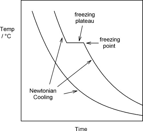
The balance here can be seen to be logically necessary. If somehow more heat were evolved, so that the temperature were raised, i.e., above the freezing point, then some metal would be obliged to remelt, absorbing that heat so that the temperature fell again to the freezing point. Likewise, if the temperature were to fall below the freezing point while molten metal was still present, some would be obliged to freeze, evolving heat to return the temperature to the freezing point and thereby restore the balance.

A typical value for the specific heat of metals is about 25 J/mol.K, while the latent heat of fusion may be about 10,000 J/mol. There is then indeed much heat to dissipate during freezing (and this is why liquid metal burns are very damaging). At the end of the freezing plateau, when there is no more liquid present, Newtonian cooling again resumes (Fig. 2.1).

•2.1 Supercooling

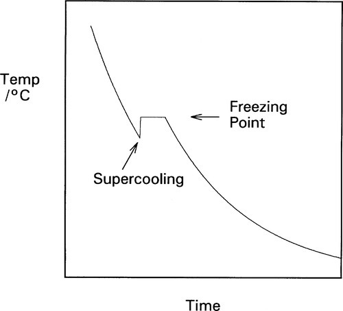
Frequently, however, freezing does not commence immediately the ‘melting’ point is reached: there may be some noticeable overshoot or supercooling (Fig. 2.2). This means that the temperature continues to decrease smoothly until crystal formation starts, when the temperature rises rapidly back to the melting point, a phenomenon called recalescence, after which the normal freezing plateau will be observed. Usually, only very little solid is required to form for this return to occur. Thus, taking the above typical figures for the specific and latent heats, some 400 g of metal would be returned to the freezing point after supercooling by just 1 K when 1 g of metal has solidified. Obviously, the temperature cannot exceed the freezing point because heat was lost during the supercooling itself, and if it did all the now-solid metal would remelt. The total heat content after recalescence must be less than that when the cooling first reached the freezing point.

An extreme example of this is very pure gallium which, if left undisturbed as it cools and in a non-nucleating sealed container such as of PTFE, can sit indefinitely in the liquid state around normal room temperature (say, ~ 23 °C), which is well below the melting point of about 29.8 °C. However, if this is disturbed such as by shaking, crystallization commences immediately, when the temperature rises promptly to the freezing point. Some explanation of this phenomenon is required.

•2.2 Energetics of crystallization

Crystalline solids are distinguished from liquids by the long-range ordering of the atoms (or molecules, remembering that there are no multi-atom molecules in either solid or liquid metals) into regular arrays. It is the change in the degree of ordering that accounts in part for the latent heat of a change of state: the local change in entropy (the thermodynamic measure of disorder) results in a large free energy change for the system.

Now, in creating a solid phase in liquid, there is necessarily the formation of a definite boundary between the two (see the definition of a phase, 8§2.3). As this boundary will be associated with an interfacial energy, γ_sl (10§1), work must be done to create it. The work of formation of that surface, W_s, is therefore proportional to the surface area or the square of the radius. To keep it simple, and illustrate the underlying principles, we can treat the particle of solid as spherical. We then have:

Ws=4πr2γs1

On the other hand, the work associated with the phase change, W_v (due to the loss of entropy), is proportional to the number of atoms involved, which is therefore proportional to the volume of the solid:

Wv=43πr3.ΔH.1‐TTm

where ΔH is the latent heat per unit volume of the solid formed, T is the actual (absolute) temperature, and T_m the melting point. The net work of formation, W_f, of the crystal of a definite size, r, is then the difference of these two terms:

Wf=Ws‐Wv

since the one is a gain, the other a loss. If this total work of formation is plotted against r (Fig. 2.3) we can see that it is not a monotonic function: it goes through a maximum and then changes sign. Thus, initially there is an increase in free energy as the crystal comes into existence and begins to grow; this is therefore unfavourable.

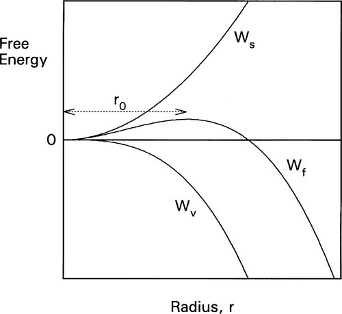
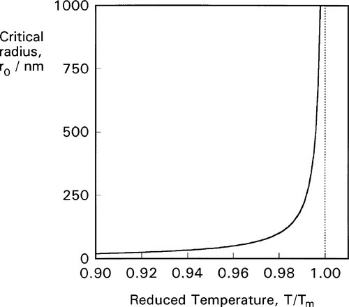
However, if a certain minimum radius (r₀) is just exceeded, the slope of the net energy curve becomes negative so that there is then a tendency for the grain of solid to grow spontaneously. This critical point is found by differentiating equation 2.4 with respect to r and setting the slope to zero. We then have:

r0=2γslΔH⋅1−TTm

From this we can see two things of interest. Firstly, when T > T_m, this critical radius, r₀, will be negative – which means that it does not exist and no crystals are formed (which is only reasonable, above the melting point). Secondly, the critical radius depends on the amount of supercooling, T_m – T: the lower the temperature the steeper the W_v curve becomes and the smaller the value of critical radius (Fig. 2.4). In fact, exactly at the melting point, the critical radius can be seen to be infinite! Hence some considerable supercooling is actually required to initiate solidification. Strictly speaking, this means that while the melting point is very well defined and realizable, the freezing point – in the absence of any solid – is not. However, once solid has formed, the equilibrium temperature is automatically obtained.

•2.3 Crystal nucleus

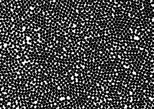
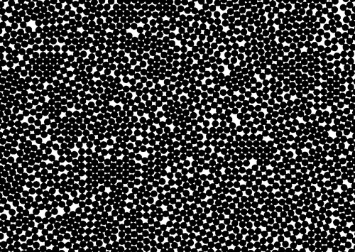
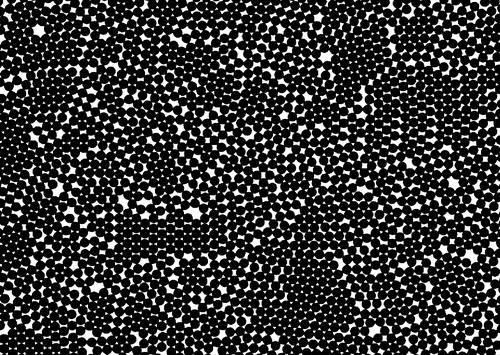
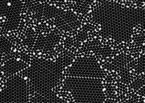
A statistical or probabilistic view of the process is helpful. Because of the rapid and continuous thermal motion of atoms in a melt, the spatial arrangement characteristic of the crystalline solid will occur spontaneously over short distances in the liquid randomly at any temperature, but be just as readily broken up or lost by further motion. The lower is the temperature, the larger such transient structures will tend to occur more readily and tend to persist longer (Fig. 2.5). Such a cluster of atoms constitutes the crystal nucleus; it may or may not grow into a crystal. Above the melting point the thermal energy of the atoms is so great that any such cluster must fly apart after only a very short time. Below the melting point, if the initial cluster survives just long enough for the accretion of enough atoms to cause it to exceed the critical radius, then growth will occur as the net energy change on freezing is then favourable.

The critical radius thus corresponds to the size of crystal nucleus at which growth and melting have an equal chance. The process could go either way at this point. For any particular cluster, the processes of addition and subtraction of atoms are random and continuous. The greater the supercooling the more centres of growth there will be throughout the liquid (as the probability of their forming is increased). With only slight supercooling, but allowing plenty of time for centres to be created, only a few will grow. The difference then is one of either many or few crystals. If many, they must be small because there is a fixed mass of metal to freeze; conversely, few nuclei yield large crystal grains. The difference between a fine- and a coarse-grained crystal structure is thus essentially dependent on the rate of cooling or, more accurately, the rate of abstraction of heat.

The fact that the formation of crystallization nuclei seems to require an input of energy needs further consideration. That is, in approaching the peak of the W_f curve in Fig. 2.3 from the left, the energy of the nucleus is greater the larger it is, and therefore more unstable with respect to the proper liquid state. It may therefore look as though a rising temperature would favour larger nuclei. But since such a rise in temperature can only increase the critical radius (equation 2.5), this is seen to be a false conclusion. It is the randomness of the formation and breakdown of the nuclei that leads to the outcome. This random, probabilistic nature of nucleation may perhaps be better understood by considering the local fluctuations in energy that may occur, even for a closed system of defined total energy.

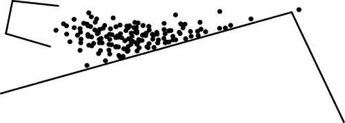
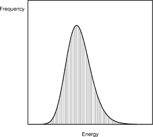
Consider a bucket of balls that are repeatedly thrown at a ramp (Fig. 2.6). The velocity with which the bucket is moved can be tightly controlled so that the total energy of the assemblage of balls is fixed. Yet it is obvious that they will not all reach the same height on the ramp for any one throw. Because of internal collisions in the group, some will rise higher than others, some not reach so far. On average, one might imagine a spread of distributions of maximum height attained on the ramp by all balls over time, much as the thermal energy of the atoms in a melt will have a range of values (Fig. 2.7). Naturally, the highest position attained by any one ball will also vary from throw to throw. Thus, on occasion, one might observe a ball go over the peak of the ramp, despite the fact that the average energy per ball is quite insufficient for this event to occur. If a ball does go over, then it must continue on down the other side, to lower and lower energy.

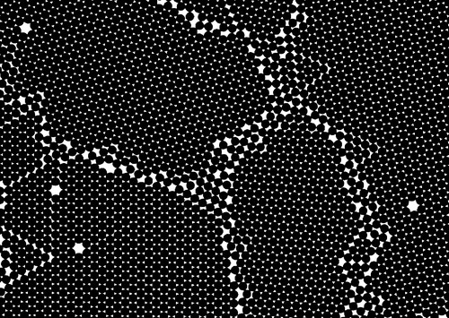
The physical counterpart of that model in the present context is as follows. In the highly-agitated liquid metal, at any given instant, there will be a random collection of nuclei of a range of sizes (Fig. 2.5a). These regions of crystal-like structure have formed by accident, and have a very short lifetime because collisions from other atoms are likely to break them apart again. The probability of finding a given size of nucleus decreases with increasing size, but it remains possible, below the melting point, for one (or more) nuclei to reach or exceed the critical radius. That is all that is required: once that condition is met, that nucleus will then grow steadily, assuming that heat continues to leave the system. The lower the temperature the greater the number of nuclei, the greater the average size of nucleus, and the greater the probability at any moment of exceeding the critical radius somewhere. Thus, crystallization is time-dependent in that the repeated ‘sampling’ of possible states (‘snapshots’) increases the probability of finding a greater-than-critical nucleus as the time interval of observation increases. It is cooling-rate dependent in that the lower the temperature the lower the critical radius and the greater the probability of finding many nuclei that can grow spontaneously.

•2.4 Homogeneous nucleation

Crystallization throughout, and within, the melt in the manner described above is termed homogeneous nucleation. The crystal nuclei are of the same material as the melt and formed from it. It is important to recognize that the nuclei of such crystals are indeed themselves crystalline, and are not formed on anything else. A liquid melt is like a violently agitated bucket of marbles: there is no long range order or structure within it. It is by chance only that locally, and only fleetingly, a few atoms may achieve an arrangement like that in the solid, crystalline material.

Thus, since this nucleation is an essentially random process (§2.3), that is, amongst other things, the locations of the nuclei are randomly distributed, it follows that the sizes of grains also have a random distribution, albeit affected by temperature gradients across the metal. This arises because a grain can only grow until it contacts an adjacent grain (which has itself been growing), when there is no more liquid available to freeze onto either side of that interface. Further, since the ‘concentration’ of nuclei also depends on cooling rate (§2.3), the mean size is greater at lower cooling rates: the total amount of metal is divided over a smaller number of grains, so their size must be greater. There is a further element of randomness: crystallographic orientation. As is detailed below (§3), crystal structures are directional in that there are layers: they cannot be structurally isotropic. Hence, as there is nothing in the melt to constrain the orientation of the layers of a nucleus, the crystallographic axes of the grain may assume any orientation in the solid. This leads to the kind of structure discussed earlier (1§2.7), and so to the effects on overall properties of polycrystalline materials that differ from single crystal behaviour.

•2.5 Heterogeneous nucleation

As with crystallization from solutions (cf. 2§6.1), heterogeneous nucleation is the process of starting the growth of crystals from the melt on, and aided by, an already solid but foreign surface. That foreign surface has, of course, a specific interfacial energy for contact with the melt so that adding atoms to it, although different, does not appreciably change either the total surface area of that contact or the net surface energy. The value of W_v therefore dominates in equation 2.4, and the critical radius may be negligibly small. In other words, its value can be rapidly exceeded (r₀ < 1 atom!) so that solidification commences immediately. The other aspect of this is the template. Most surfaces are rough at the atomic scale, with steps in the faces of crystals, defects of various kinds (see Fig. 2§7.3) that provide ready niches for further atoms to settle into. Once such an atom has been added there still remains a step which can accommodate another, and so on. So long as the imposed spacing is sufficiently close to the natural spacing of the metal freezing out, the crystal will grow readily.

•2.6 Exponential decay

Reference was made at the beginning of the section to the exponential form of the temperature-time plot for Newtonian cooling. The explanation of this will now be set out to complete the picture.

There are many systems in which the rate that a quantity, say B, declines with respect to time is proportional to the current value of B. This is written as a differential equation in the following way:

−dBdt=KB

where k is the constant of proportionality and the leading negative sign indicates that it is a decreasing function. The question to be answered is: how does the value of B actually vary with time? The answer is given by integrating this expression, and since it is so important this will be set out rather than just stating the result. Rearranging to separate the variables:

−dBB=k.dt

so that:

−∫B0B1B.dB=k.∫0tdt

From standard tables this is:

lnB0−lnB=kt

or

lnB=lnB0−kt

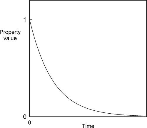
which gives a straight line plot (Fig. 2.8), or:

B=B0e−kt

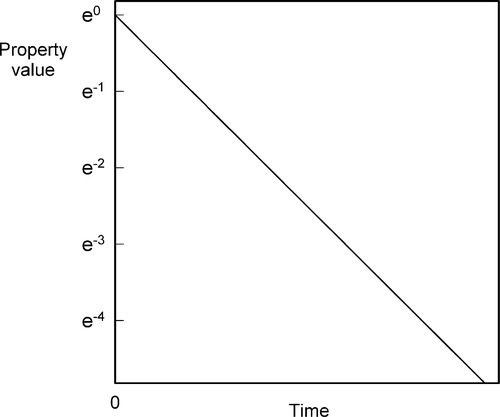
which is the exponential decay function (Fig. 2.9).

The simplest example, perhaps, is that of radioactive decay where B is the number of unstable nuclei in the sample. It is also the form for a so-called first-order chemical reaction where B is the concentration of the reacting species. If B is substituted by ΔB, meaning the difference B – B_∞, where B_∞ is the value that is eventually attained, we have the form for Newtonian Cooling (Fig. 2.1, §2.7); B then of course is temperature. Similarly, the deformation of a Kelvin-Voigt body (4§5) is obtained from the same analysis where B is replaced by the strain in the system. Lambert’s Law is derived likewise, only instead of time as the ‘elapsed’ variable we now have distance traversed. This applies to X-radiation in matter (26§3), visible light through filters (26§5.2) and similar systems.

•2.7 Cooling curves

The determination of a cooling curve is the simplest form of thermal analysis. The typical basic form of the experiment is shown in Fig. 2.10. A sample of the material is heated to some appropriate starting temperature, and then the temperature is monitored as it cools in an undisturbed manner. Heat (Q) is lost to the surroundings at temperature T_R (across the tube wall, for example, in Fig. 2.10) according to the temperature difference (ΔT = T – T_R, sometimes called the temperature excess), the area of the interface, A, and the efficiency with which that heat is transferred across the interface, what is called the “exterior conductivity”, H (i.e. in W/K/m²). So, we can write:

−dQdt=AH⋅ΔT

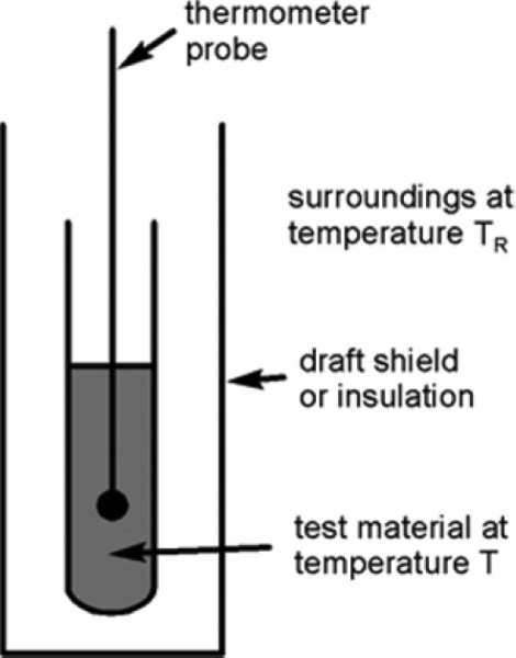
The effect on the temperature of the sample that this loss of heat has depends on the specific heat, cp,¹ and the mass of the material:

Q=ΔTcpM

However, we are usually not in a position to know A, H or c_p (which may vary with temperature), and M is arbitrary, so we can substitute for Q from equation 2.13 into the left-hand side of equation 2.12 and write:

−dT